Chapters


Regression Definition
If you’ve ever heard about popular conspiracy theories, you might be astounded by the level of detail groups have gone to in order to explain the unlikely relationships between events or phenomena. While on the surface conspiracy theories and statistics may seem like they’re on opposite ends of the spectrum, they have both arisen out of the well-documented tendency of humans to see patterns everywhere.
Patterns can be predictable, but they can also be very subjective. One dataset, for example, can be interpreted in a vast number of ways by researchers or students depending on their interests, abilities, and more. The beauty of statistics is that it has many different tools for discovering and analysing these patterns.
Regression is one of these tools. The most basic form of regression is linear regression, which investigates the relationship between one dependent variable and one or more independent variables. Linear regression strives to investigate the relationship between different variables and whether some can be used to predict another.
Ordinary least squares is the most common type of linear regression. Ordinary least squares seeks to minimize the squared errors in the model. The equation for OLS regression is:
[
y ; = hat{alpha} ; + hat{beta}*x
]
The OLS estimators,  and
and  , can be calculated with the following equations:
[
hat{beta} ; = frac{sum_{i=1}^n (x_{i}-bar{x}) (y_{i} - bar{y})}{sum_{i=1}^n (x_{i} - bar{x})^2} = frac{sigma_{xy}}{sigma_{x^2}} = rho_{xy} frac{sigma_{y}}{sigma_{x}}
]
[
hat{alpha} = bar{y} - hat{beta}*bar{x}
]
Correlation Definition
You might recognize the word correlation. While the statistical term is often used in media as a sure-metric for a relationship between two variables, it might not mean what you think it means. Take a look at the graph below.

For each observation, we have ice cream sales on a given day and shark attacks on the same day. Notice that as ice cream sales go up, so do shark attacks - in fact, it looks like there is a near perfect correlation. While correlation does measure the strength of the relationship between two variables, it does not mean there is cause and effect between them.
| Type | Description | Formula |
| Pearson’s correlation coefficient | Describes the strength of a linear relationship between two variables |  |
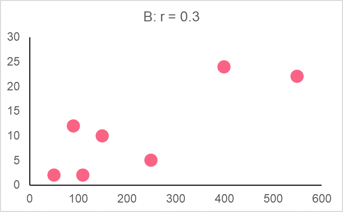
The best way to learn how to interpret correlation is by looking at correlation coefficients besides their graphs. Below are a series of graphs plotting two variables.
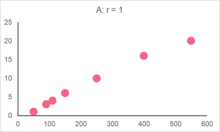


| Image |  | Interpretation |
| A | 1 | Perfect positive correlation, as one variable increases, so does the other |
| B | 0.3 | Low positive correlation |
| C | 0 | No correlation, no relationship between the two variables |
| D | -0.3 | Low negative correlation |
| E | -1 | Perfect negative correlation, as one variable increases, the other decreases |
We can also use regression models as a way to predict for the event’s we’ve modelled. Check out the table below to understand the two main categories of predictions.
| Type | Definition | How it’s Done |
| Extrapolation | The estimation of a value that is outside the data set range | Plug the desired value into the regression formula |
| Interpolation | The estimation of a value that is inside the range of the data set | Plug the desired value into the regression model |
Problem 1
Calculate and interpret the correlation coefficient of the two variables below.
| Person | Hand | Height |
| A | 17 | 150 |
| B | 15 | 154 |
| C | 19 | 169 |
| D | 17 | 172 |
| E | 21 | 175 |
Problem 2
The graph below represents each individual’s weight and corresponding blood pressure. Recall in previous sections the formulas for calculating a regression line. Using the correlation coefficient and regression line, interpret the graph.
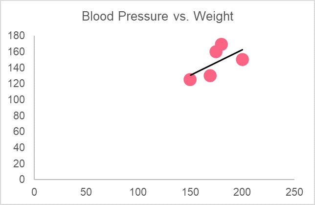
| Person | Weight | Blood Pressure |
| A | 150 | 125 |
| B | 169 | 130 |
| C | 175 | 160 |
| D | 180 | 169 |
| E | 200 | 150 |
Problem 3
The following graph shows the regression model for age and salary. You are given the following regression model:
[
y = -14,448.8 + 2,552.5*x
]
Using the information given below to give an example of interpolation and extrapolation based on this model.
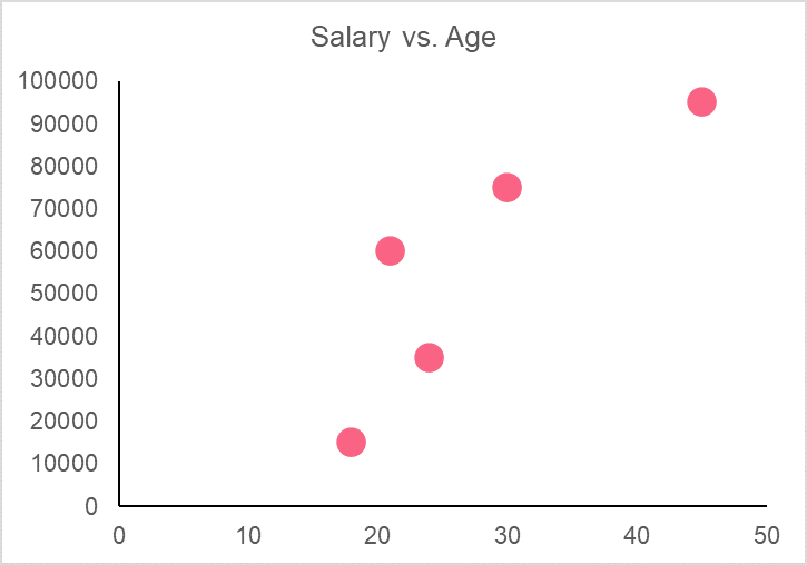
| Person | Age | Salary |
| A | 18 | 15000 |
| B | 21 | 60000 |
| C | 24 | 35000 |
| D | 30 | 75000 |
| E | 45 | 95000 |
Solution Problem 1
In order to solve this problem, let’s take it step-by-step.
- Calculate the means
- Subtract the means from every value
- Multiply and square these subtracted values
- Sum these multiplied and squared values
| Person | Hand | Height | 
| 
|  |  |  |
| A | 17 | 150 | -0.8 | -14.0 | 11.2 | 0.6 | 196.0 |
| B | 15 | 154 | -2.8 | -10.0 | 28.0 | 7.8 | 100.0 |
| C | 19 | 169 | 1.2 | 5.0 | 6.0 | 1.4 | 25.0 |
| D | 17 | 172 | -0.8 | 8.0 | -6.4 | 0.6 | 64.0 |
| E | 21 | 175 | 3.2 | 11.0 | 35.2 | 10.2 | 121.0 |
| Average | 17.8 | 164 | Total | 74.0 | 20.8 | 506.0 |


Lastly, you plug everything into the formula. Check out the table below for this calculation.
| Formula | Result |
 | 74 |
 | 20.8 |
 | 506 |
| Formula |  |
The formula gives us a correlation coefficient of 0.72, which is a high, positive correlation. Meaning that in this data set, as height increases, so does hand height.
Solution Problem 2
First we calculate the correlation coefficient.
| Person | Weight | Blood Pressure |
|
| | | |
| A | 150 | 125 | -24.8 | -21.8 | 540.6 | 615.0 | 475.2 |
| B | 169 | 130 | -5.8 | -16.8 | 97.4 | 33.6 | 282.2 |
| C | 175 | 160 | 0.2 | 13.2 | 2.6 | 0.0 | 174.2 |
| D | 180 | 169 | 5.2 | 22.2 | 115.4 | 27.0 | 492.8 |
| E | 200 | 150 | 25.2 | 3.2 | 80.6 | 635.0 | 10.2 |
| Average | 174.8 | 146.8 | Total | 836.8 | 1310.8 | 1434.8 |
Which yields a correlation coefficient of,
[
frac{836.8}{sqrt{(1310.8*1434.8)}} = 0.61
]
Next we calculate the regression line.
 |  = 18.94 = 18.94 |
 |  = 18.3 = 18.3 |
 |  = 0.64 = 0.64 |
 |  = 35.21 = 35.21 |
 | y = 35.21 + 0.64x |
This information is summarized below.

Weight and blood pressure have a moderate, positive correlation. Looking at the slope, this means that as weight goes up by 1 kg, blood pressure goes up by 0.64.
Solution Problem 3
To give an example of interpolation and extrapolation, simply plug in values within and outside the data set into the regression model. Below are some examples
| Age | Result | Type |
| 24 | 46,811.02 | Interpolation |
| 60 | 13,8700.80 | Extrapolation |
Did you like this article? Rate it!


