Chapters


Descriptive Statistics

| Hours Spent Studying | Exam Score |
| 3 | 70 |
| 4 | 80 |
| 5 | 90 |
With descriptive statistics, we can calculate two types of measures and illustrate descriptive properties of the dataset.
| Description | Example | |
| Measures of central tendency | Measures the centre of the dataset, such as mode, median and mean | The mean exam score is: 80 |
| Measures of spread | Measures how far spread the data, such as the variance and standard deviation | The standard deviation of the exam score is: 10 |
| Descriptive visualizations | Illustrates descriptive characteristics, such as pie charts, bar charts, line graphs | You can plot these points on a line graph |
Correlation Definition
The correlation coefficient, also known as the Pearson product-moment correlation coefficient, is a descriptive statistic. It measures the strength of the linear relationship between two variables. A linear relationship is one that can be explained by a linear equation. Take a look at the two images below.

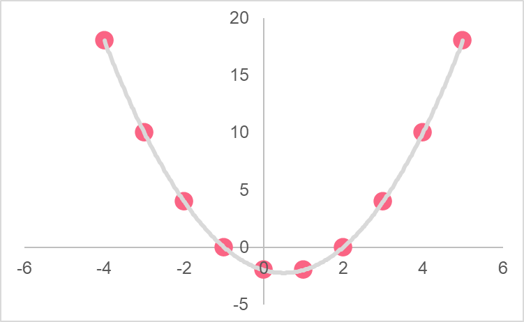
The variables in the first line graph have a relationship that can be explained by a linear equation, which is plotted by the straight line. The variables in the second line graph, on the other hand, have a relationship that follows the shape of a parabola. This type of relationship can be described by a quadratic equation.
Correlation Formula
In order to calculate the correlation, you should first understand the definition of covariance. Take the image below as an example. This image depicts the values of two variables on a line graph: the grade on the final exam and hours of attendance.
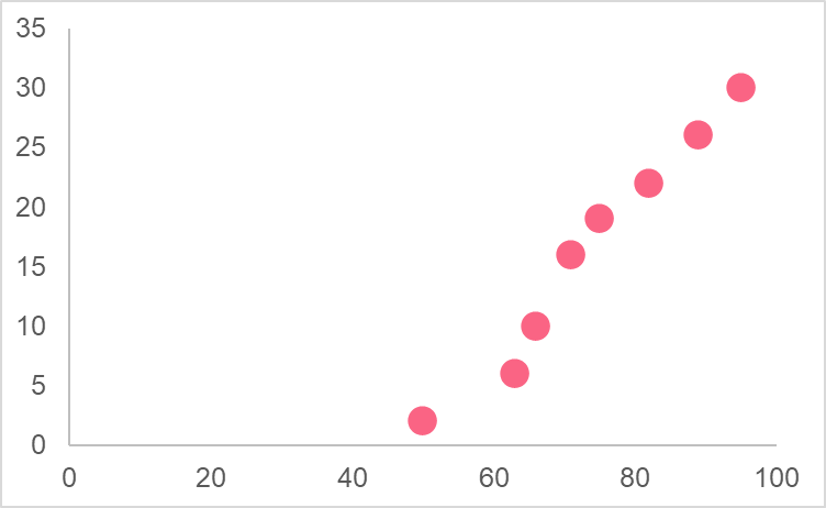
This pattern is described as a positive pattern: as the number of hours of attendance increases, the number of points on the final exam also increases. Here, we can say that the two variables are moving together. When we describe the movement of two variables, we are using the covariance. In statistics, the covariance tells us how two variables move together and it is calculated as the following.

We can use the covariance of two variables to calculate the correlation of two variables. The formula for the correlation is the following.

The table below describes the elements within the formula.
| Element | Description |
 | The sample covariance of x and y |
 | The standard deviation of x |
 | The standard deviation of y |
| n | The sample size of the data |
Types of Correlation
The correlation coefficient can tell us how strongly related two variables are. However, how exactly can we interpret this correlation coefficient? In other words, is there any way we can tell what is a strong and weak relationship?
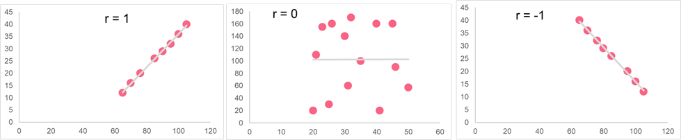
The image below shows the general rules of thumb for interpreting the correlation coefficient. Everything in between these numbers, however, is a bit subjective. However, there are some general guidelines you can adhere to, which are summarized in the table below.
| -1 | -0.8 | -0.5 | -0.3 | 0 | 0.3 | 0.5 | 0.8 | 1 |
| Perfect negative correlation | Strong negative correlation | Moderate negative correlation | Weak negative correlation | No correlation | Weak positive correlation | Moderate positive correlation | Strong positive correlation | Perfect positive correlation |
When the terms positive and negative are referred to in statistics, they don’t mean the same thing as they do in regular life. In statistics, positive and negative generally refers to the direction.
| Type | Movement | Interpretation |
| Positive | Together | If one variable decreases, the other one decreases too (and vice versa) |
| Negative | Opposite | If one variable decreases, the other one increases (and vice versa) |
Correlation versus Causation
It is quite common to see people mistake correlation and causation. This isn’t without reason - the two can seem pretty similar. However, if we take a look back at the formula for the correlation, we can see that these two notions don’t have too much alike. Causation is defined as one thing causing or producing an effect on another thing. When you turn on the light switch, this causes the light to turn on.
However, correlation is simply the covariance over the multiplication of the standard deviations of the x and y variables. It tells us about the direction of the movement of x and y scaled by the standard deviations. It can only tell us about the linear association between two variables, not about whether one causes the other. One classic example is hand size and height - the two are very strongly correlated. However, this does not mean that hand size causes height - there are a number of factors that link the two.
Correlation Example
Let’s run through an example of correlation together. Let’s take the data set from the first example.
| Hours Spent Studying | Exam Score |  |  |  |  |  |
| 3 | 70 | -1 | -10 | 10 | 1 | 100 |
| 4 | 80 | 0 | 0 | 0 | 0 | 0 |
| 5 | 90 | 1 | 10 | 10 | 1 | 100 |
| Mean = 4 | Mean = 80 | Total | 20 | 2 | 200 |
Plugging it in, we get the following:
\[
r(x,y) = \dfrac{20}{\sqrt{2*200}} = 1
\]
Did you like this article? Rate it!


