Chapters
Matrix multiplication and statistics intersect in many different ways. There is nowhere this is more apparent than in ordinary least squares regression. Using matrices to form the OLS equation instead of regular numbers can be more convenient when you have a large amount of data. Try the problem below in order to test what you already know about matrices and OLS. Keep in mind that this problem is based off of Solution to Problem of Regression 8. See the solution in the guide below.


Problem 9
In the previous problem (Solution to Problem of Regression 8), you were asked to format the data into matrices. Now, using these matrices, find the regression model equation and interpret the results in terms of what this means for the shop owner.
Least Squares Matrix Equation
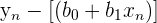
Recall that OLS regression is a form of linear regression that strives to reduce the sum of squared errors. Take a look at the equations below to refresh your memory on OLS regression.
 | Simple linear regression |
 | Multiple linear regression |
 | Residual |
OLS regression can be quite simple to calculate when there are only one or two independent variables. However, these operations are time consuming and can often be impractical when dealing with more than two independent variables.
This is where the matrix form of OLS regression becomes very helpful. Take the following system of equations.
| Points | Equation | y | x |
 | 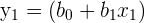 |  |  |
 | 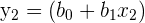 |  |  |
| ... | ... | ... | |
 | 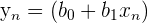 |  |  |
Instead of writing all equations, we can write them in matrix form:
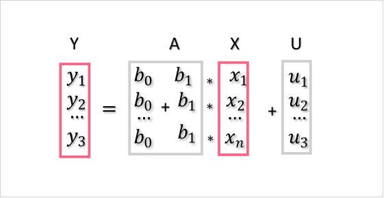
Where the matrices simply become.

Matrix Multiplication
In order to solve this matrix equation, we should first go over matrix multiplication. A matrix is simply an array of numbers.
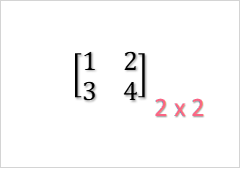
Each matrix has dimensions, which are written as 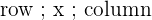 . When multiplied by a scalar, or a single number, you simply multiply each entry in the matrix by the scalar.

This would be calculated in the following way.
| 3*4 | 12 |
| 3*0 | 0 |
| 3*10 | 30 |
| 3*-2 | -6 |
However, a matrix multiplied by another matrix requires finding the “dot product” of a matrix. For example, you have two matrices.

The dot product here is simple:

In order to multiply matrices, you need to multiply the first row with the first column. Next, you would multiply the first row with the second column. This matrix multiplication would result in the following.
| (1*4) + (2*10) | 24 |
| (1*0) + (2*-2) | -4 |
| (3*4) + (4*10) | 52 |
| (3*0) + (4*-2) | -8 |
Keep in mind that when multiplying matrices, only those that have matching inner values can be multiplied.

In the example above, we were able to multiply the matrices because they were (2x3) x (3x2). Both have the same  values, resulting in an (n x p) matrix, which in this case is a (2x2).
Transpose Matrix
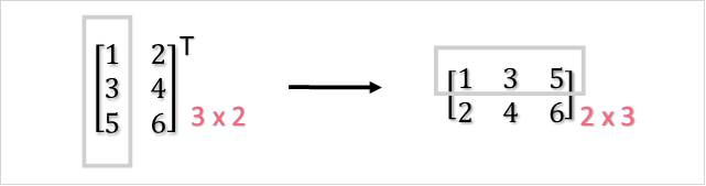
Now that you understand matrix multiplication, let’s go over the transpose of a matrix. Transposing something is to make two or more things exchange places. When you transpose a matrix, all rows become columns. For example, if you have a 3x2 matrix, it will become a 2x3.
| Column 1 | Column 2 | |
| Row 1 |  |  |
| Row 2 |  |  |
| Row 3 |  |  |
The above matrix, for example, has entries  , where n is the row value and k is the column value. The transpose of this matrix would become the following, where reflects the original order:
| Column 1 | Column 2 | Column 3 | |
| Row 1 | | | |
| Row 2 | | | |
Therefore, the rule for transposing any matrix is that any (n x k) matrix will become (k x n).
Inverse of a Matrix
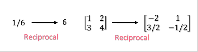
In order to find the inverse of a matrix, you should understand why we’re interested in inverse matrices in the first place. Just like you can find the reciprocal of a fraction, you can also find the inverse of a matrix.
In order to find this matrix, you should understand the concept of an identity matrix.
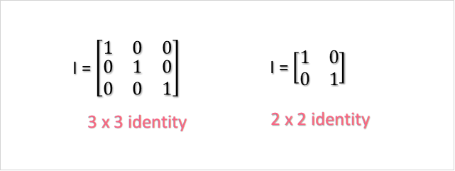
Check out the properties of an identity matrix below.
| Square | A square matrix has the same number of rows and columns |
| 1’s on diagonal, 0s elsewhere | The diagonal of a matrix is the line of numbers that runs diagonal from it starting from the top left and ending at the bottom right |
| Any size | An identity matrix can be any size, ranging from 2x2 to 100x100 and beyond |
The inverse of a matrix is said to exist if and only if:

The easiest inverse to find is that of a 2x2 matrix because it follows the formula:

Notice how the diagonal is switched and c and b become negative. The determinant is simply ad-bc.
If you have a bigger matrix, you can use what is called an “augmented matrix”, which is basically the original matrix next to its inverse.

The goal is to perform elementary operations to the rows in order to get the right side as an identity matrix, which will make the right side the inverse. Take the following as an example.

As you can see, we would solve for the matrix in these steps.
| Row 3 | = row 3 - row 1 |
| Row 1 | = row 1 - row 2 |
| Row 3 | = row 3 + row 2 |
| Row 2 | = row 2 divided by 2 |
| Row 3 | = row 3 divided by 3 |
| Row 1 | = row 1 + row 3 |
| Row 2 | = row 2 - (½)*row 3 |
To check that we have the inverse, we simply multiply A and  to see if we get the identity matrix.

The SSE
The sum of squared errors is how we can determine how accurate our model is. When calculating the sum of squared errors, or SSE, for matrices, you first need the following formula.

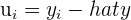
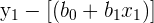
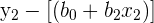
The matrix U is made up of the residuals for each equation in the system of equations. Remember that, in order to find the residual, you have to do the following.
| Residual | Formula | Simplified Formula |
 |  |  |
 |  |  |
| ... | ... | ... |
 |  |  |
This means that, in order to find the SSE, you first have to find the OLS equation in matrix form. Once you find this matrix equation, you simply plug in the x values to see what y value your model estimates. Next, you subtract this estimated y value from the actual observed y value from your data set for the same x value. This is your residual, which can then be formatted into a matrix.

Solving OLS Matrix Equation
In order to find the solution to this OLS equation through matrices, recall that you first need to solve for the matrix A. The A matrix will give us both the intercept and the slope of the equation, which is why it’s so important. First, calculate the inverse of the first part of the A formula.


After solving for the inverse, you need to plug the inverse into the rest of the A equation. This gives us the following y-intercept and slope:

As you can see, the slope is negative. This means that as the demand goes up, the price goes down by -0.196. Keep in mind that normally, demand is the y variable because we would rather explore the demand at different price points rather than the other way around.
| Price | Demand |  |  |
| 120 | 110 | 122.44 | -2.44 |
| 125 | 100 | 124.4 | 0.6 |
| 130 | 90 | 126.36 | 3.64 |
| 135 | 45 | 135.18 | -0.18 |
| 140 | 20 | 140.08 | -0.08 |
After calculating the residuals, you plug them in to the SSE equation to see that the error is quite low. The model predicts price pretty well.

Did you like this article? Rate it!


