


What is Regression?
If you’ve been in any sort of maths class, read the news or are interested in keeping up with the current pandemic, you’ve probably seen a chart like this:
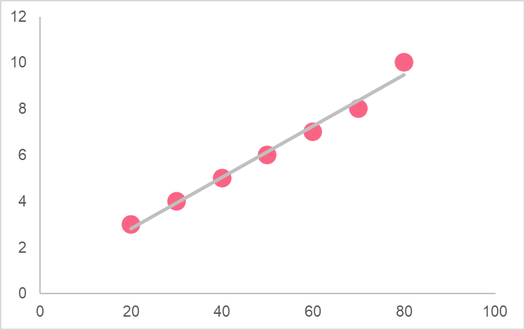
When you see two numerical variables plotted along with a line, you are looking at a regression model. A regression model is a statistical model that seeks to measure the strength of the relationship between two variables. This relationship is then used to try and predict future events.
The line above is an example of a regression line, which is an equation that describes the relationship between the explanatory and response variables.

As you can see from the image above, the explanatory variables are those you are using to try and predict your response variable. Response variables are those that respond to, or are dependent on, other variables.
As you can see, response variables can also be called independent variables. Explanatory variables, on the other hand, can also be called independent variables. With classic linear regression, there is only one response variable with one or more explanatory variables.
Correlation Interpretation
Unless you’ve been hiding under a rock, you’ve probably heard of the word correlation. This is because correlation is one of the most popular statistics out there. The golden rule of correlation is that correlation does not equal causation.
Causation is defined as the action of causing something. In statistics, as with most disciplines, nothing is ever known for certain. This is because statistical models cannot possibly account for all the different possible variables or external effects that can cause even one singular event. If this sounds a bit crazy, check out the graph below.
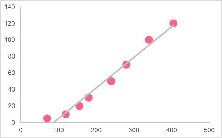
As you can see, this graph plots the relationship between ice cream sales and sunburns. The correlation coefficient between these two variables is 0.99. This high correlation coefficient suggests the following:

This means that as ice cream sales go up, so do sunburns. The correlation here simply tells us that there is a strong, positive relationship between these two variables. Does it mean that ice cream sales cause sunburns? Definitely not, in fact the variable that ties these two together is in fact increased sunny days.
SLR
So far, we’ve taken a look at some basic concepts behind regression. Let’s dive into the most common regression type, which is known as simple linear regression. Simple linear regression, or SLR, is known as simple linear regression because it only has one response variable and one explanatory variable.

To understand the two equations above, you should recall the difference between a population and a sample. A population is the group of people, places, ideas or things you want to study. A sample, on the other hand, is taken from the population and is used to estimate characteristics of the population.
An example of this is the effect of a fertilizer on flower growth. The population could be all the flowers in a forest, a country, or even in the whole world. However, because it is impossible to measure the effects of this fertilizer on all the flowers in our population, we would take a sample of that population and study it instead.
MLR
Multiple linear regression, known as MLR, is an extension of SLR. As you probably guessed, the only difference between MLR and SLR is the fact that MLR has more than one explanatory variable. Taking our example from above, this could be studying the effects of fertilizer and temperature on plant growth.

Taking a look at the equations above, you can see that this time, we have added more explanatory variables to our equation. We use our sample to estimate the true population parameters. These parameter estimates are known as the regression coefficients. Take a look at the equation, graph and metrics below.

| Parameter | Regression Coefficient | P-value |
| bo | 30 | 0.004 |
| b1 | 1.2 | 0.032 |
| b2 | 3.5 | 0.001 |
This is an example of a standard output you will get whenever performing MLR. As you can see, there is two main components: the coefficient and its corresponding p-value. With a significance level of alpha = 0.05, all of the parameters are statistically significant. This means that they can be used to predict plant growth.
The coefficients, on the other hand, indicate the increase that plant growth would exhibit with a increase in one unit of the parameter. The table below interprets these coefficients.
| Regression Coefficient | Interpretation |
| 1.2 | An increase in one unit of the x1 variable leads to a increase of 1.2 in the y variable |
| 3.5 | An increase in one unit of the x2 variable leads to a increase of 3.5 in the y variable |
Problem 1
Here, we’ve covered the fundamental aspects of regression models. Specifically, we’ve shown you their function and interpretation. Now, it’s time to put what you’ve learned into practice. This problem deals with these basic concepts - if you get stuck, the solution to the problem is at the bottom.
The following model has been made in order to be able to predict hot dog sales using the number of people attending a sports game.

You’re interested in interpreting the model and using the model to be able to predict hot dog sales for the next game. In order to do so, a single linear regression model has been run and has returned the following output.
Solution Problem 1
In this problem, you were asked to interpret the given model and use it to make a prediction. Below, you will find a summary of what each element in the model means.
| 1 | Sales | The response variable is hot dog sales |
| 2 | 100 | The constant of the model |
| 3 | 1.6 | Hot dog sales increase by 1.6 given an increase of 1 person attending |
| 4 | People | The explanatory variable is the amount of people who attend |
As you can see, while simple linear regression may seem too basic, its model can actually tell us quite a lot of information. To predict the number of hot dog sales when 3,000 people are in attendance, you simply need to plug the number into the equation.
This gives you a total of 4,900. If we interpret this number, this means that if 3,000 people attend a match, we predict that 4,900 hot dogs will be sold. This is important if we know other elements, such as the price and cost of making each hot dog. This could give us insight into the revenue.
Did you like this article? Rate it!


