Chapters


What are Inferential Statistics?

| Inferential | Descriptive | |
| Definition | Statistical analysis that predicts the future using the dataset | Statistical analysis that illustrates or measures data included in the dataset |
| Measures | -Regression -Hypothesis tests | -Central tendency (mean, mode) -Spread (standard deviation, variance) |
| Variable Types | Numeric and Categorical | Numerical and Categorical |
| Example | Regression analysis between test score and hours spent studying | Calculating the mean test score for different schools |
Regression Definition
You have probably heard of regression in many different contexts. This is because regression analysis is one of the most widely used tools of inferential statistics. Regression analysis is defined as the process of measuring the relationship between two or more variables.

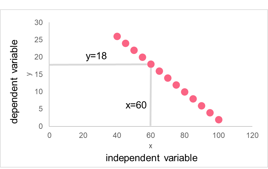
The image above is a graph containing the two types of variables in regression analysis: independent and dependent variables. Notice that there is a pattern between these two variables. This pattern can be captured with a regression model, which models the linear relationship between two variables.
| Independent Variable | Dependent Variable | |
| Definition | The variable that we use to predict our dependent variable | The variable that responds to the independent variable |
| Type | Numeric or categorical (known as a ‘dummy’ variable) | Numerical, can only be categorical when using a special type of regression called logistic regression |
| Other Names | Explanatory variable | Response variable |
Simple Regression Formula
As mentioned, linear regression can be used to model the relationship between two or more variables. When a linear regression involves only one independent and one dependent variable, this is known as simple linear regression, or SLR.
The graph above is the same as the one before, with the only difference being the line running through the observed data points. This line is known as a regression line. The regression line is calculated based off of the following formula.

The reason why there are two formulas has to do with the fact that one is the formula for the population while the other is a formula for the sample. Recall that a population contains all the things we want to study, which means that we rarely have access to all the data from the population. The sample, on the other hand, is a subvert of the population. With the sample, we can find an estimation of the true population regression model.
| Population | Sample | |
| Response Variable | The population dependent variable | The sample dependent variable |
| Explanatory Variable | The population explanatory variable | The sample explanatory variable |
| Constant | The value of the population dependent variable when all independent variables are zero | The value of the sample dependent variable when all independent variables are zero |
| Regression coefficient | The population parameters | The sample estimates of the population parameters |
| Error | The part of y not explained by x | Is assumed to be zero |
SLR Estimate Formulas
Many SLR models are run using some program or software. Meaning, programs such as R or Python take the data in your model and run the regression model automatically, calculating all regression coefficients and statistics. Many people, when learning statistics, start by calculating regression estimates by hand.
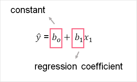
In the image above, you can see that there are two parameters that we estimate using SLR. The first is the y-intercept, which is the value of y when all x’s are zero. The formula can be seen below.
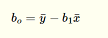
The following table describes each element in the formula
| Element | Description |
 | Mean of y |
 | The regression coefficient |
 | Mean of x |
As you can see, we need to first calculate the sample regression coefficient before calculating the intercept. Below, you can find the formula for .
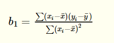
The following table contains the explanation for the formula.
| Element | Description |
 | The ith observation of x |
| The mean of x |
 | The ith observation of y |
| The mean of y |
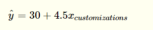
In order to find the full regression model, all you need to do is simply plug the calculated constant and regression coefficient into the model. Take the following scenario as an example.
| Element | Description |
| y | Shoe price |
 | 30 |
| 4.5 |
| x | Number of customizations |
In the above example, the slope and regression coefficient have already been calculated. The SLR model would therefore look like this:
Problem 1
In this section you learned about the differences between descriptive and inferential statistics. You are interested in understanding the differences between what analysis you can do on a data set. You are given the data set below, which comes from a restaurant on the beach. This restaurant is interested in knowing what the relationship is between the number of soups sold and the weather. Classify the types of analysis you can do on this data set based on the differences between inferential and descriptive statistics.
| Soup Sales | Temperature |
| 24 | 2 |
| 15 | 10 |
| 8 | 17 |
| 5 | 27 |
Solution to Problem 1
In this problem, you were asked to:
- Understand the differences between the two branches of statistics
- Write down some analysis you can do based on these two branches
The first step in solving this problem is knowing what the main differences are between inferential and descriptive statistics. First, descriptive statistics uses the information within the data set in order to describe what the data looks like. On the other hand, inferential statistics uses the data set to try to make inferences about data points outside of its range.
Next, we can classify the different analysis in the table below.
| Inferential | Descriptive |
| Simple linear regression | Measures of central tendency: mean, median, mode |
| Hypothesis testing | Measures of spread: variance, standard deviation, range |
| Modelling | Descriptive visualizations: pie chart, bar chart, etc. |
Problem 2
In the previous example you were asked to describe the types of analysis you could conduct based on the two types of statistics. Next, using the same data, you are asked to conduct a regression analysis. Build a simple linear regression model based on the formulas provided. Next, describe how this model would look on the following chart.

Solution to Problem 2
In this problem, you were asked to build a regression model. First, you need to calculate the mean. Next, subtract the mean from all observations in your data set and
| Temperature | Soup Sales |  |  |  |  |
| 2 | 24 | -12 | 11 | 144 | -132 |
| 10 | 15 | -4 | 2 | 16 | -8 |
| 17 | 8 | 3 | -5 | 9 | -15 |
| 27 | 5 | 13 | -8 | 169 | -104 |
| Mean = 14 | Mean = 13 | Total | 338 | -259 |
Next, we plug it into the equations for and :
\[
b_{1} = \dfrac{-259}{338} = -0.766
\]
\[
b_{o} = 13 - (-0.766*14) = 24
\]
Finally, we get the following regression:
\[
\hat{y} = 24 - 0.766(temperature)
\]
This model would be a line on the graph above.
Did you like this article? Rate it!


