Chapters
Formatting ordinary least squares equations into matrix form can be a very efficient way of solving for a least squares regression line. This is because, instead of taking every value individually, the values are taken as a whole column. Try to apply what you’ve learned from our other guides to the problem below. If you struggle to come up with a solution or are learning about this concept for the first time, read through this guide.


Problem 8
A shop owner is interested in understanding the demand of certain goods in her store based off of the price. In order to help the store owner, you’re tasked with conducting a simple regression analysis. Given the following data set, your first task is to explain how to format these observations into matrices along with the benefits of using matrices in statistics.
| Price | Demand |
| 120 | 110 |
| 125 | 100 |
| 130 | 90 |
| 135 | 45 |
| 140 | 20 |
OLS Linear Equation
Recall that ordinary least squares, or OLS, is a type of regression analysis that strives to reduce the sum of squared residuals. OLS can take on two forms, summarized in the table below.
| Simple Linear Regression | Multiple Linear Regression |
| SLR | MLR |
 |  |
| One dependent variable | One dependent variable |
| One independent variable | Two or more independent variables |

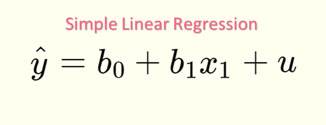
To understand OLS regression, you have to understand the formulas involved. There are two major formulas, which are the least squares linear equation and the residual formula.
| The least squares linear equation |
 | The y-intercept, the value of y when all x’s are zero |
 | The regression coefficients, which tell us how one independent variable relates to y |
 | The estimation of the error term, otherwise known as the residual |
To understand the reason why OLS tries to reduce the sum of the squared error, look at the image below.
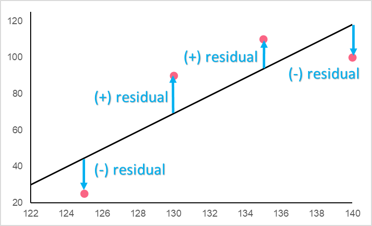
The residual is the difference between the actual observed value  given by an
  and the predicted value
  , also known as y-hat, given by the same . The best line, naturally, would be the regression line with the least distance between the actual observed y values and the predicted y values. However, how can you compare residuals when they have different signs?
| Example | Sign | Interpretation |
 |  positive positive | Overestimated |
 |  negative negative | Underestimated |
As you can see, while the magnitudes are both 15, if we didn’t square the residuals the negative sign would deflate the total sum. This is why residuals are squared.
OLS Matrix Equation
If we were to solve this equation using OLS, we would have to utilize the steps and equations summarized below.
| Step | Description | Formula |
| 1 | Write down the OLS equation | |
| 2 | Find the slope | 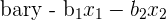 |
| 3 | Find all  | 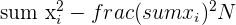 |
| 4 | Find all  |  |
| 5 | Find all parameters  |  |
 | ||
| ... |
This can be time consuming, especially if we had more than just two independent variables. This is where matrices come into play. Think about the points  in your data as a system of equations.
| Points | Equation |
 | 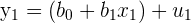 |
 | 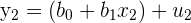 |
| ... | ... |
 | 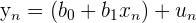 |
Taking this system of equations, you can reformulate this data into matrix form.

In this form, we only have two steps, summarized below.
| Step | Description | Formula |
| 1 | Write down the OLS equation | 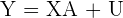 |
| 2 | Solve for the matrix A |  |
Solving OLS Matrix Equation
By multiplying the matrices out, you can see the resulting system of equations from earlier. Take the first two entries, as an example.

This would multiply out to be the following.
 | |
 | |
Here, we would like to solve for as it contains the y-intercept and slope information. Because matrices can’t just be moved around on either side of the equals sign, we have to perform special operations known as taking the transpose and inverse of a matrix, resulting in the following formula.

The transpose of a matrix is simply flipping a matrix from, for example, being 2x3 to 3x2, like below.

The inverse of a matrix, on the other hand, involves elementary row operations to get from  ot
ot  .
.

OLS Matrix Equation Example
In order to get used to matrix notation, let’s go through an example. You have data on height and heart beats per minute, which are illustrated below.
| Height | Heart Beat |
| 160 | 55 |
| 169 | 50 |
| 174 | 70 |
| 180 | 80 |
You know this could be written in the following equations:
| (160, 55) |  |
| (169, 50) |  |
| (174, 70) | 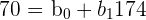 |
| (180, 80) | 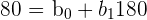 |
Instead, we can now write them in matrix notation.

OLS Matrix Equation Problem
In this problem, you were asked to format the data set into matrix multiplication. First, let’s start by separating the data into a system of equations. Doing this will help us visualize which numbers we have to place in each matrix.
| Y | X | Formula |
| 120 | 110 | 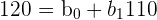 |
| 125 | 100 | 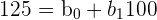 |
| 130 | 90 | 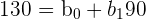 |
| 135 | 45 |  |
| 140 | 20 | 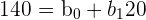 |
Now that we have the data formatted this way, it’s easy to see what to put in which matrix. Now, we just follow the formula from above, where each matrix contains the different variables and/or parameters necessary. Below, you'll see what this should look like.
The benefit to this is that it will be a lot easier to solve by hand, and computationally, than without matrices. As you can see, instead of having to find the solutions to the formulas of about 5 or more metrics, we can now just solve for A through less complicated matrix multiplication.
Did you like this article? Rate it!


