Chapters
The Gauss-Markov theorem is one of the most important concepts related to ordinary least squares regression. In order to fully understand the concept, try the practice problem below. If you’re having trouble solving it, or are encountering this concept for the first time, read this guide for a detailed explanation, followed by a step-by-step solution.


Problem 6
A classmate of yours is having trouble understanding what makes ordinary least squares, under the Gauss-Markov theorem, the best linear estimators as opposed to all the other estimators. Given the following example, explain what BLUE estimators mean and why they are important.
A sample is taken from a population that measures the money the observed companies spend on advertising and the amount of sales that they make in one month.
OLS
Recall that OLS is ordinary least squares, which is a regression model that strives to reduce the space between the regression line, or the predicted y values, and the actual observed y values. The equation of a simple OLS is the following.
[
hat{y} = b_{0} + b_{1}x + u_{i}
]
Where  is the estimated y value and the regression coefficients are b_{0}, the intercept, and
  , the slope. The
  term is the residual, which is the distance between the regression line and the predicted value.

We take the square of each residual in order to account for negative residuals, which is when the predicted y value is higher than the observed y value. This is why OLS is called ordinary least squares, because we are trying to minimize the sum of all of the squared residuals.
Under certain conditions, these linear estimators are said to be the best, unbiased linear estimators, otherwise known as the acronym BLUE.
What are Estimators?
Recall that whenever we’re trying to predict phenomena, we work with samples. A sample is a group of values we observe from a population. A population includes the objects, ideas or places we would like to study. Because it is always near impossible to measure the entire population, people take samples from the population and use these samples to make estimation on the population.
The real values from the population are called population parameters and the estimates of those parameters calculated from the sample are called statistics. This leads to the central question: what makes a good estimator?
While we have presented OLS as the linear regression equation that is most commonly used, you have to wonder why the majority of people have picked OLS estimators over the many other linear estimators we could have used. To judge a good estimator, we have to look at three characteristics:
| Unbiasedness | Does not under or over-estimate the population parameter |
| Consistency | As the sample size increases, the estimator converges closer to the population parameter |
| Efficiency | Has the smallest variance of all possible estimators |
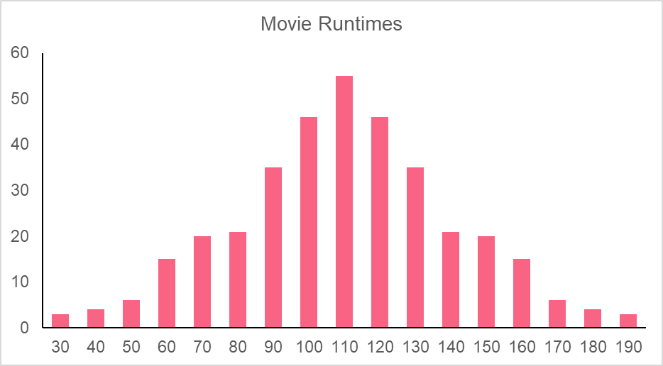
In order to understand these characteristics, let’s look at a frequency distribution.
Recall that the Law of Large Numbers, of LLN, states that with enough samples, the sample mean approximates or equals to the true population mean. Using this principle of the LLN, we can see that our estimate of the parameter , with enough samples, approximates the true population parameter  .
.
The unbiasedness of an estimator looks like the frequency distribution below. With enough samples from the population, we arrive at a group of estimates for each sample. This means that the mean estimator does not over or underestimate the true population parameter .

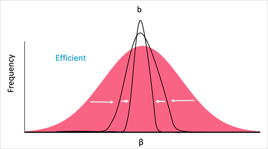
Consistency, on the other hand, means that with increased samples, the mean converges closer and closer to the true population parameter, which we can see in the shape of the distribution. This narrower shape indicates less variance.

Finally, efficiency can be represented below, where the higher the samples, the less variance there is - ultimately leading to an estimator with the least variance, which is deemed the most “efficient.”
What is the Gauss-Markov Theorem?
The Gauss-Markov theorem states that, under certain assumptions, an OLS regression results in unbiased linear estimates that have the smallest variance out of all possible linear estimators. These assumptions can be found in the table below.
| Assumption Met | Assumption Not Met | Description |
 |  | Linear in parameters - note that while the x value can be non-linear, our parameters ( ) cannot be non-linear ) cannot be non-linear |
 are random sample are random sample | are not random sample | If each individual in the same population is equally likely to be picked for the sample, a sample is random |
 |  | Zero conditional mean of the error term - given  we cannot know whether will be above or below the mean we cannot know whether will be above or below the mean |
Weak correlation between  |  | No perfect collinearity - the independent variables cannot have a high correlation, for example if you have  by meters and by meters and  meters squared meters squared |
 |  not constant not constant | Homoskedasticity - constant variance meaning the variance doesn’t vary systematically (with a pattern) with x |
 |  | No serial correlation - errors need to be independent of one another |
What does BLUE mean?
If the OLS regression model meets these six assumptions, the estimators of that regression model are said to be BLUE. The table below explains this acronym.
| B | The best estimator in terms of efficiency and consistency |
| L | Linear |
| U | Unbiased |
| E | Estimator |
In other words, under these six assumptions, the model has the best, linear, unbiased estimators of all possible estimators.
Gauss-Markov Problem Step by Step
The Gauss-Markov theorem is one that states that, under certain conditions, our set of linear estimators will be BLUE. Take the example that was given: a manager wants to understand how the amount of advertising impacts sales and so takes a sample from their database.
What is stopping us from simply using any estimator? For example, perhaps the manager notices that every time she spends 1,000 pounds more on advertising, she doubles her sales. This could be considered an estimator of its own.
However, there could be a better way to estimate her sales data - which is by finding the linear equation from her sample’s points. This is a better way of estimating her data and predicting how many sales she’ll make at different price points for advertising. This is because a linear model allows for better extrapolation and interpolation.
Extrapolation is performed when you use your model in order to predict for x and y values outside of your dataset. Interpolation, on the other hand, is performed when you use your model to predict for x and y values inside the range of your dataset. While many people think of extrapolation as the more important tool for analysis, interpolation can actually help you see how good your model is at predicting your target variable with data you have already.
Under the 6 classic linear regression model assumptions, or the Gauss-Markov assumptions, this linear model is the best out of all possible linear models. With an independent and random sample, along with homoscedasticity, no perfect collinearity, and all the other G-M assumptions, your data and model can lead to the best, unbiased, linear estimators.
This is important because you can be assured that your model is capturing the true population parameter even better than any model. Ultimately, this leads to less variability and more reliable results. Think about how important that could be to a manager, whose use of the best model can mean the difference between a couple hundred pounds in loss to a couple hundred thousand.
Did you like this article? Rate it!


