Chapters
Simple linear regression is one of the most commonly used statistical analysis tools in the field. In order to understand the ideas that make up simple linear regression, try to solve the following problem by reviewing what you already know. Read through this guide if you’re unsure about or are encountering this concept for the first time.


Problem 4
There are two variables that need to be studied: weight loss and days spent exercising one month. You are given a data set in which individuals have been asked the number of days they exercise for more than half an hour in one month. What kind of regression model can you use here? What are the results of this regression given the data set below. Interpret the model’s estimators.
| Exercise Days | Weight Loss (in kg) |
| 0 | 4 |
| 4 | 1 |
| 8 | 1.5 |
| 12 | 2 |
| 16 | 4 |
| 20 | 5 |
| 24 | 2 |
What is SLR-OLS?
Simple linear regression, or SLR, is a regression analysis that involves only one explanatory and one response variable. The definitions of these two variables can be found below.
| Explanatory or Independent Variable | The variable manipulated by the investigator, the one that will explain the variance in the dependent variable | The explanatory variable of time spent studying on an exam |
| Response or Dependent Variable | The variable that responds to the manipulation of the independent variable, the one that responds to changes in the independent variable | With the explanatory variable of time spent studying, the response variable of the exam score |
SLR analysis yields a regression model between two variables that can be used to make predictions, or estimations, about observations inside and outside the range of the data used to make that regression model.
OLS Explained
One important component of conducting a simple linear regression analysis is ordinary least squares, otherwise known as OLS. OLS is a method for estimating the unknown parameters of a linear regression model.
In every regression analysis, there are independent and dependent variables that are being studied from a dataset. In the majority of cases, this dataset is a list of observations for the dependent and independent variables from individuals that make up a sample. This sample is taken from the population because it is extremely rare to have data from the entire population.
Recall that the population is made up of all the individuals, objects or ideas that you want to study. The measurements of a population are called parameters, while the measurements of a sample are called statistics.
When it comes to linear regression, there are many different ways we can try to estimate these population parameters with our sample statistics. The reason why OLS is so vital to linear regression is because it minimizes the difference between the observations in the dataset and the predicted responses of the linear regression model.
The formula for the regression line, estimators and residuals of OLS can be found in the table below.
| Element | Formula | Description |
| Slope | 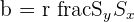 | Slope of the regression model |
| y-intercept | 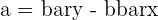 | The y-intercept of the regression model |
| Model |  | The regression model |
| Residual | 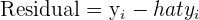 | Difference between observed y and predicted y |
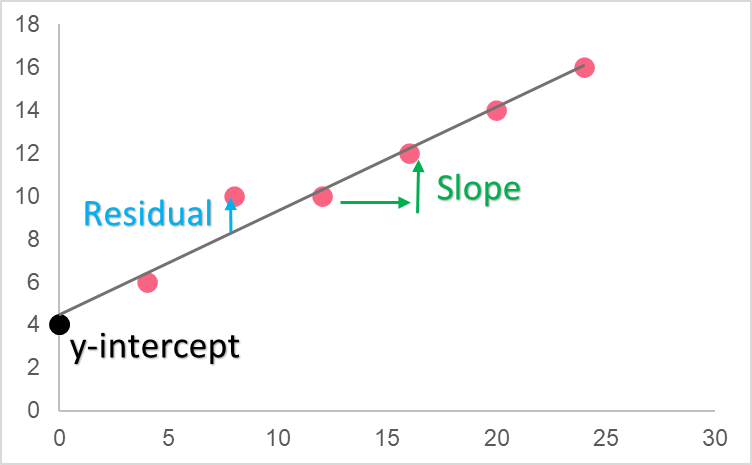
The reason behind the ordinary least squares regression model is that it is the linear model for which there is the least distance between the line and the predictors. In other words, it is the regression line for which all residuals, or the difference between the data set and the predicted data points, are the least.
Meaning of OLS
As you can see, the linear regression line includes residuals, which are the estimates of the error. The error is the same concept as the residuals, except for the actual population, making the residual a statistic, or estimate of the true population parameter.
Rearranging the formula, we can see that the residual is simply
[
y_{i} = alpha + beta x_{i} + u_{i} ; rightarrow ; u_{i} = y_{i} - alpha - beta x_{i}
]

Because the best linear regression line is one that reduces the distance between its predictions and the actual observed values from the sample, the goal would naturally be to want to reduce the residuals for all points in the sample. Because residuals can be positive or negative, depending on whether the line under or overestimates y, we square them. This is so that we can compare the magnitudes of the positive residuals with those of the negative residuals equally.


Because we want to reduce the square of each of these residuals, we call this linear regression model ordinary least squares.
Interpretation of Regression Line
To interpret the linear regression line, you have to understand what the estimators within the formula mean. The slope of the regression model is called the regression coefficient while the y-intercept is simply the y-intercept. Take a look at the table below for an interpretation of each estimator.
| Estimator | Value | Interpretation |
| Slope | Weight = 0 + 100(Height) | The weight here is in kg while the height here is in meters. This means that an increase in one meter will result in an increase of 100 kg to height. |
| y-intercept | Weight = 0 + 100(Height) | Recall that the y-intercept is the point on the y-axis for which the x value is zero. This means that, in this model, if the height were zero, the weight would be 0 kg. This makes sense, as you can’t weigh something when you don’t have any height. |
| Slope | Sales = 40 - 5(Price) | Here, the price is in pounds and the sales are per unit. Because the slope is negative, this means that for an increase of 1 pound in the price there would be a decrease of 5 units sold. |
| y-intercept | Sales = 40 - 5(Price) | This is an example of a y-intercept that is nonsensical. While you can interpret it as being the sales for when the price is 0, it wouldn’t make any sense for the price to be 0. This is why, before interpreting the y-intercept, think about the normal range for the x variable. |
OLS by Hand
| Observations | Exercise Days | Weight Loss |   |   |  |  |  |
| 1 | 4 | 4 | -12.0 | 1.2 | -14.6 | 144.0 | 1.5 |
| 2 | 8 | 1 | -8.0 | -1.8 | 14.3 | 64.0 | 3.2 |
| 3 | 12 | 1.5 | -4.0 | -1.3 | 5.1 | 16.0 | 1.7 |
| 4 | 16 | 2 | 0.0 | -0.8 | 0.0 | 0.0 | 0.6 |
| 5 | 20 | 4 | 4.0 | 1.2 | 4.9 | 16.0 | 1.5 |
| 6 | 24 | 5 | 8.0 | 2.2 | 17.7 | 64.0 | 4.9 |
| 7 | 28 | 2 | 12.0 | -0.8 | -9.4 | 144.0 | 0.6 |
| Mean | 16.0 | 2.8 | Total | 18.0 | 448.0 | 13.9 |
[
r_{xy} = frac{18}{sqrt{448*13.9}} = 0.29
]
[
S_{x} = sqrt{frac{448}{7}} = 8
]
[
S_{y} = sqrt{frac{13.9}{7}} = 1.4
]
Now we calculate the slope.
[
b = 0.29 * frac{1.4}{8} = 0.04
]
Next we plug this in to find the y-intercept.
[
a = 2.8 - 0.04*16 = 2.14
]
Finally, the model is:
[
y = 2.1 + 0.04x
]
Where the slope tells us the change in weight loss given a change of 1 unit of exercise days.

Did you like this article? Rate it!


