Chapters


Regression Definition
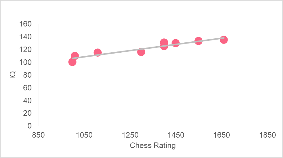
Take a look at some of the most common statistics involved in regression. Continuing the example illustrated by the image above, a regression model has been built between chess player ratings and their corresponding IQs.
| R Squared Value | The explanatory variable(s) explain (R squared)% of the variance in the response variable |
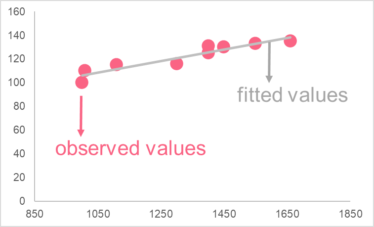
| Regression Line | The regression line is the plotted “fitted” values |
| Fitted Values | The y values that the regression model predicts |
CLRM
The classical linear regression model has several assumptions that go with it, which can be summarized below.
| Assumption | Description |
| 1 | Linear in parameters |
| 2 | Simple is picked at random |
| 3 | Zero conditional mean of the error term |
| 4 | No perfect collinearity |
| 5 | No heteroskedasticity |
| 6 | No autocorrelation |
Under these assumptions, the Gauss-Markov theorem holds. The Gauss-Markov theorem states that if a certain set of assumptions are met, the estimators in the regression model are the best, linear, unbiased estimators. This is also known as being “BLUE.”
Checking these assumptions before interpreting your regression model is vital. These assumptions are necessary in order for the model you’ve created to be valid.
MLR
Recall that multiple linear regression is just an extension of simple linear regression, or SLR. The main difference is that MLR models have more than one explanatory variable. For this reason, they are even more common than SLR models. After all, one event or thing is rarely fully able to be explained by only one variable.

Taking a look at the graph above, we can see that in addition to IQ score, a chess player’s rating is also correlated with their weekly practice times. Because both IQ and practice time are potentially great predictors of chess rating, we can use them in an MLR together.
The three most important components of an MLR output are: the p-value of the estimators and model, the regression coefficients and the R-squared value.
| Component | Description |
| R-Squared value | A measure of how good the explanatory variables are at predicting the response variable |
| P-value of F-statistic | A measure that tells us if the explanatory variables are good predictors of the response variable. If the p-value is statistically significant, this means that we’ve picked good explanatory variables |
| Regression Coefficients | These tell us how the response variable increases or decreases in response to an increase in one unit of the explanatory variable |
| P-value of the regression coefficients | This measure tells us if the explanatory variables are statistically significant. Meaning, if they predict the response variable or not. |
MLR with Dummy Variables
A dummy variable is a categorical variable that can be used in regression. This dummy variable takes on numerical values that represent the different categories in the variable. The most classic example of a dummy variable is gender, which can be seen in the table below.
| Category | Dummy Variable |
| Female | 1 |
| Male | 0 |
While we typically only include true numeric variables in our regression, as we can’t calculate maths with words such as female or male, we can work around this by using dummy variables. This allows us to use statistical methods such as MLR without limiting ourselves to quantitative variables.
Other examples of dummy variables can be success and failure, or yes and no, or even qualitative variables with more than one category, such as direction (north, east, south, west).
Interpretation of Dummy Variables
Take a look at the image below.

Notice that if we include dummy variables in our MLR model, we use delta instead of beta. Another difference that occurs when we use dummy variables is related to the categories included in our regression. If there are k number of categories, we always include only k-1 in our regression.
This is done so that we can use the category that is left out as a reference value. You leave out one category only when you are including a constant in your model.

This means that the interpretation for dummy variables is a bit different than for numerical variables. The constant term, Bo, represents the value of y value for the second category here. In other words, when IQ and practice hours remain constant (which we just set to 0), the average value of y is simply equal to Bo for males. Females, on the other hand, have an average of y equal to Bo plus delta1 - meaning, the female average is higher than the male average by delta1.
Problem 1
In this section, we reviewed single and multiple linear regression, touching upon the basic concepts involved in each. In addition, we also discussed the definition of a dummy variable and its interpretation. This problem will test you on these concepts and if you have trouble finding the solution, the next section will walk you through it.
You have been asked to interpret a multiple linear regression model that we saw in a previous example. A multiple linear regression analysis has been run and yielded the following output.
\[ chess \; rating = 1000 + 4.5 \; IQ + 1.3 \; practice + 0.76 \; gender \]
Interpret each element of the MLR model, paying special attention to the dummy variable. Just to refresh your memory, the dummy variable has two categories: female, coded as 1, and male, coded as 0.
Solution to Problem 1
In this problem, you were asked to interpret the regression model. In the table below, you can see the interpretation for each element of the model.
| 1 | y | Chess rating is the response variable |
| 2 | 1000 | The constant is 1000 |
| 3 | 4.5 | Everything held constant, if IQ increases by one point, chess rating increases by 4.5 |
| 4 | 1.3 | All other variables held constant, if weekly practice hours increase by 1, chess rating increases by 1.3 |
| 5 | 0.76 | Everything held constant, the mean chess rating for women is 0.76 points higher than that of males |
Did you like this article? Rate it!


