Chapters


What is Regression?
Simple Linear Regression
Simple linear regression, or SLR, is a long name for a very simple concept: a regression model that has only one independent and one dependent variable. Check out the image below, which summarizes the differences between the two types of variables.

Recall that in statistics, the phenomena you want to measure can involve people, things, places or ideas. Check out the table below for some examples.
| People | How many people eat ice cream ever year? |
| Places | Has this park changed over time? |
| Things | How tall do trees go at high altitudes? |
| Ideas | What political ideas do different groups of people prefer? |
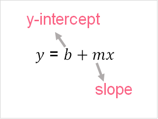
In order to measure these things, an SLR model can be utilized. SLR models can be calculated either by hand or by software. Ultimately, the resulting model will resemble the equation below.

SLR Interpretation
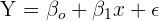
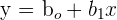
Because people can rarely measure all the things, people, places or ideas involved with their question, we often use samples drawn from the population and use these sample measures as estimates for the population. This is why you will often see two formulas for SLR models.
While the general ideas of the two equations are the same, you should keep in mind that there are some fundamental differences between the two. The table below gives a brief overview of how to interpret each.
| Population SLR | Sample SLR |
 |  |
| y is the response variable of the population |  is the estimate of the response variable is the estimate of the response variable |
 is the constant is the constant |  is the estimated constant is the estimated constant |
 is the population parameters for the explanatory variables is the population parameters for the explanatory variables |  is the estimated regression coefficient is the estimated regression coefficient |
| x is the independent variable of population | x is the independent variable of the sample |
 is the error term of the population is the error term of the population | The error is assumed to be zero |
R-Squared Interpretation
The r-squared value is a value that represents the proportion of the variation in the y variable that is explained by the x variable. In other words, it measures how well the model accounts for the movements in y. This value is typically calculated automatically in any program used to run regression. However, the r-squared value can also be calculated by hand.
The formula above shows the standard calculation for the r-squared value. In order to understand this formula, each element is described below.
| Element | Description |
| R^2 | The r-squared value |
| RSS | Sum of squared residuals |
| TSS | Total sum of squares |
As you can see, the r-squared value is the ratio between the RSS to the TSS. Take a look at the table below in order to find the formula and definition for both of these elements.
| Element | Formula | Definition |
| TSS |  | How much variation the response variable has |
| RSS |  | How much of the variation in the response variable not explained by the model |
SLR Estimators
In order to estimate any SLR model, you can typically do it on a variety of programs by simply inputting the data and clicking a few buttons. However, you can also calculate simple linear regression by hand. In order to do this, you need to calculate the following.
| Element | Formula |
|  |
|  |
As you can see, the first step in calculating any regression model is to calculate the mean of both the dependent and response variables. Next, you will have to calculate the regression coefficient. Finally, you plug in the regression coefficient into the equation for the constant.
Problem 1
The following information involves a data set containing two variables. These two variables involve the average amount of hours spent studying outside of class per week and the final grade in the class. This data is plotted on the graph below, where the line represents the regression model associated with the data.
Describe the relationship between the two variables. Using the regression model, make a prediction for the final grade of someone who studied 30 hours per week.
\[
\hat{y} = 29.22 + 2.25x
\]

Solution to Problem 1
and . The interpretation is the following:
- In increase in 1 hour of study leads to an increase of 2.25 points
- 29.22 is the final grade when there are zero study hours.
In order to predict for 30, we simply need to plug it into the regression equation.
\[
\hat{y} = 29.22 + 2.25(30) = 97
\]
Problem 2
In the previous example, the task involved interpreting a regression model. This time, you are asked to calculate a regression model and interpret it. You are given four pieces of information, written below.
- Mean of y = 66.2
- Mean of x = 22
 = 358
= 358 = 805
= 805
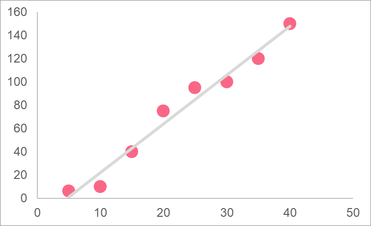
After calculating the regression model, make a prediction for an x value that is equal to 40. The graph below, which shows the plot of the data points, may help you in interpreting the model.

Solution to Problem 2
In order to solve for the model, we simply have to plug in the given information into the formulas for the constant and regression coefficient.
\[
= = \dfrac{805}{358} = 2.25
\]
\[
= = 66.3 - (2.25*22) = 16.73
\]
The regression model is:
\[
\hat{y} = 16.73 + 2.25x
\]
To estimate for a value equal to 40, simply plug the number in.
\[
\hat{y} = 16.73 + 2.25(40) = 107
\]
Did you like this article? Rate it!


