Chapters


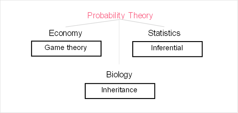
What is Probability Theory?
| Concepts | Difficulty Level |
| Simple probabilities of an event | 1 |
| Conditional probability & Bayes’ Theorem | 2 |
| Sensitivity, specificity, likelihood ratio | 3 |
| Probability using distributions | 4 |
This section will cover some elements in all of these levels of difficulty.
Random Variable
Random variables are the basic building block in probability theory. Random variables are distinct and should not be confused with traditional variables. The image below shows illustrates some of the major differences between the two.
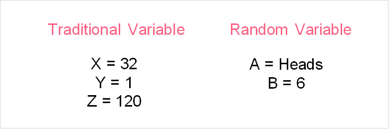
As you can see, traditional variables are quite different from random variables. The table below explains these differences.
| Type | Definition | Notation | Example |
| Traditional Variable | A symbol for an unknown value | Lower case letters | Height, density |
| Random Variable | A variable whose outcome is unknown | Upper case letters | Roll of a dice, toss of a coin |
While traditional values are typically measured or calculated, random variables are unknown until either an experiment is run or through the use of the probability.
Expected Value
Let’s say that a factory produces rain jackets and is interested in understanding whether or not the production of these jackets are uniform. The first step the factory takes is to measure the length of each rain jacket, giving them the following.
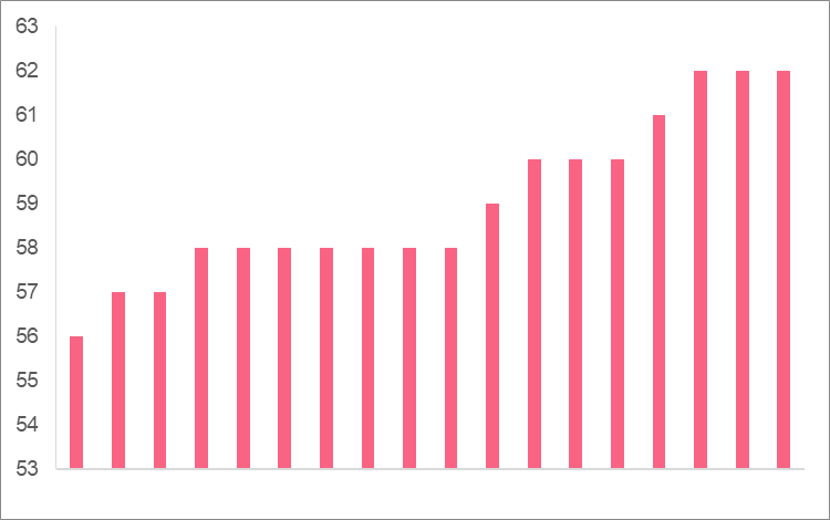
This sample of 18 jackets gives them an idea of the average size of the jackets they produce. In other words, this sample mean tells them what jacket length they can expect from the factory.
Similarly, the expected value of a random variable can be thought of as similar to the mean of a traditional variable. Take a deck of cards as an example.
| Card Value | Number Included in Deck |
| 1 | 10 |
| 2 | 5 |
| 3 | 3 |
| 4 | 2 |
The formula for expected value can be seen below.

The elements in the formula are broken down in the table below.
| Element | Description |
| E[X] | Expected value of random variable X |
 | Mean |
 | Sum of all x’s times their probabilities, where X is taken to equal x |
In this case, the expected value for the deck of cards would be:
| Card Value | Number Included in Deck | Probability |  |
| 1 | 10 |  | 0.5 |
| 2 | 5 |  | 0.5 |
| 3 | 3 |  | 0.45 |
| 4 | 2 |  | 0.4 |
| Sum | 20 | 1.85 |
In other words,

Probability Density Function
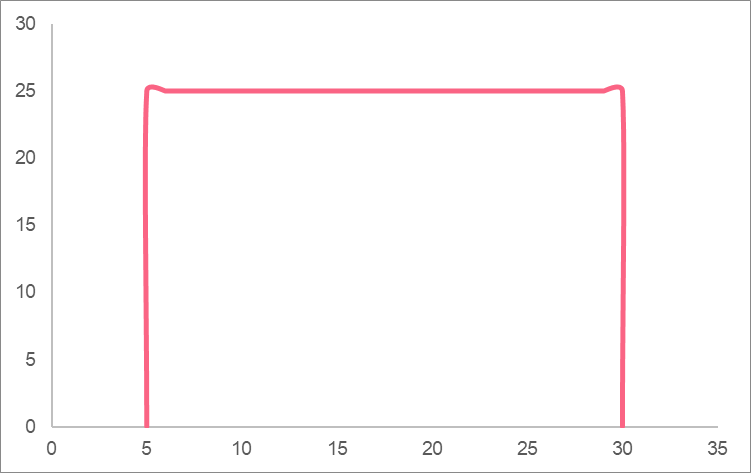
A probability density function is a function that lets us know the shape of the distribution. A probability distribution is a visualization that tells us what the probability of each value of a random variable is. Distributions can be uniform, exponential or normal.
| Type | |
| Uniform |  |
| Exponential |  |
| Normal |  |

Cumulative Distribution Function
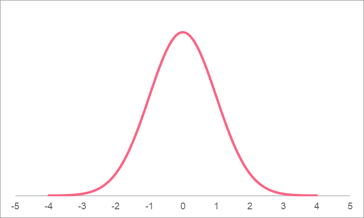
A cumulative distribution function is a function that represents the area between two points under the curve on a continuous distribution. Recall that a probability distribution tells us the probability of a value occurring for each value a random variable can take on. The most common example of a probability distribution is a normal distribution.
The cumulative distribution function, or CDF, of the distribution above could tell us what the cumulative probability is between the two points, as shown by the highlighted area.
Types of Distributions
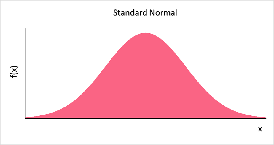
There are many different types of probability distributions. This is because different random variables have different values and different probabilities assigned to those values. Think about a coin toss, which only has two possible values: heads or tails. The probability of getting heads or tails is different as the number of trials increases. This distribution looks a lot different to the probability distribution of, say, the height of people in a population. The two probability distributions we’ll talk about here are listed in the table below, along with their formulas and examples.
| Standard Normal | N(, ) ) |  | IQ scores in a population |
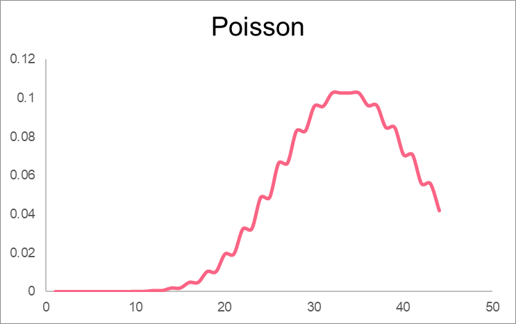
| Poisson | Po( ) ) |  | Number of customers at a gas station per hour |

Problem 1
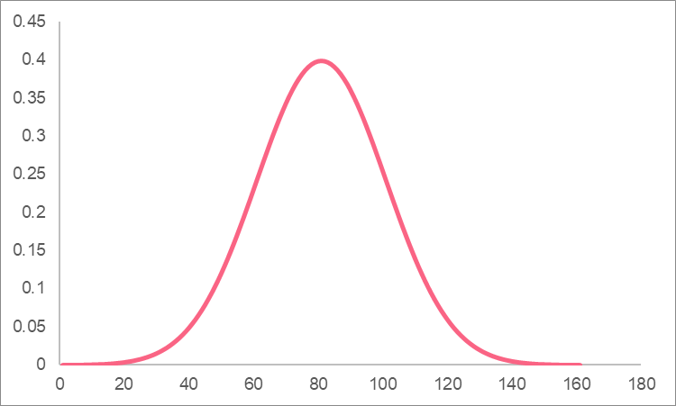
You are interested in calculating the probability that someone has an IQ score of 110 given the following information.
| Population average | | 100 |
| Population standard deviation | | 15 |
Solution 1
In order to calculate the probability of an IQ of 110, we need to first calculate the z-score, which is the formula in the table in the previous section.
\[
z-score = \frac{110-100}{15} = 0.667
\]
In order to see what the probability of this z-score is on a standard normal curve, we have to look at a z-table. Since we’re interested in a left tail z-score - that is, all the probabilities up to 110 - we look at a left-tail z-table.
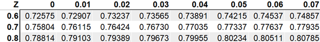
This gives us a probability of 0.7454.
Problem 2
You need to create an annual report that gives people information on how many customers enter their store per day. In order to do this, you measure the following information.
- The mean number of people per day is 15
Given this information, calculate the probability of 9 and 20 people entering the store on two separate days.
Solution 2
In order to calculate the probability of people entering the store, we simply plug in the mean, which is  , into the equation for a Poisson distribution. Keep in mind Poisson distributions are those that deal with probabilities in time.
\[
\frac{15^{9} e^{-15}}{9!} = 0.324
\]
For 200 customers, this probability is the following
\[
\frac{15^{20} e^{-15}}{20!} = 0.0418
\]
Did you like this article? Rate it!


Using facebook account,conduct a survey on the number of sport related activities your friends are involvedin.construct a probability distribution andbcompute the mean variance and standard deviation.indicate the number of your friends you surveyed
this page has a lot of advantage, those student who are going to be statitian
I’m a junior high school,500 students were randomly selected.240 liked ice cream,200 liked milk tea and 180 liked both ice cream and milktea
A box of Ping pong balls has many different colors in it. There is a 22% chance of getting a blue colored ball. What is the probability that exactly 6 balls are blue out of 15?
Where is the answer??
A box of Ping pong balls has many different colors in it. There is a 22% chance of getting a blue colored ball. What is the probability that exactly 6 balls are blue out of 15?
ere is a 60% chance that a final years student would throw a party before leaving school ,taken over 50 student from a total of 150 .calculate for the mean and the variance
There are 4 white balls and 30 blue balls in the basket. If you draw 7 balls from the basket without replacement, what is the probability that exactly 4 of the balls are white?