Chapters
In the previous section on standard scores, we introduced you to the concept of standardizing data and using its standardized value to understand how typical it is for a data set with a given mean and standard deviation. In this section, we’ll dive deeper into z-scores and show you how to use a z-table.


Z-Scores
Employing the classic example used when teaching z-scores, let’s examine the idea of test taking. If you take a test that is out of 100 points and only score 50 points, you may be tempted to interpret that as a bad score. After all, many point systems are based on an absolute scale. Meaning, no matter how a class performs, 50 points generally considered to be a failing grade.
If this isn’t clear to you, think about what would happen in the opposite scenario, where a grade is based on a relative scale. Instead of being scored out of 100 points, let’s say your teacher decides to base the test on the highest grade in the class. This is a relative scale because it is graded relative to how the class performs. If the highest grade in the class is 55 points, you might have actually performed extremely well.
This example is meant to illustrate the problem with raw scores, which are simply unaltered data points or calculations form your data set. Your raw score of 50 out of 100 or 55 can’t actually tell us how well you did when compared to the entire class. You could have scored the average amount of points, or perhaps have been the worst.
In statistics, raw scores can be transformed in order to be more comparable. One method of transformation is percentiles - which is discussed in other sections of this guide - where your grade can be compared to the percentage of people scoring above and below you.
Another method is called standardization, which is the basis of z-scores. Standardizing data removes whatever units that data set is in and allows each data point to be compared in terms of standard deviations. Recall the formula for standardization below, which happens to also be the same formula for finding the z-score.
| Sample Z-Score | Population Z-Score |
| \[ Z = \frac{x - \mu}{\sigma} \] | \[ z_{i} = \frac{x - \bar{x}}{s} \] |
Continuing from our example, let’s say the mean score for the test taken is 74 and the standard deviation is 8. Calculating the z-score, we would get the following.
\[
z_{i} = \frac{50 - 74}{8} = -3
\]
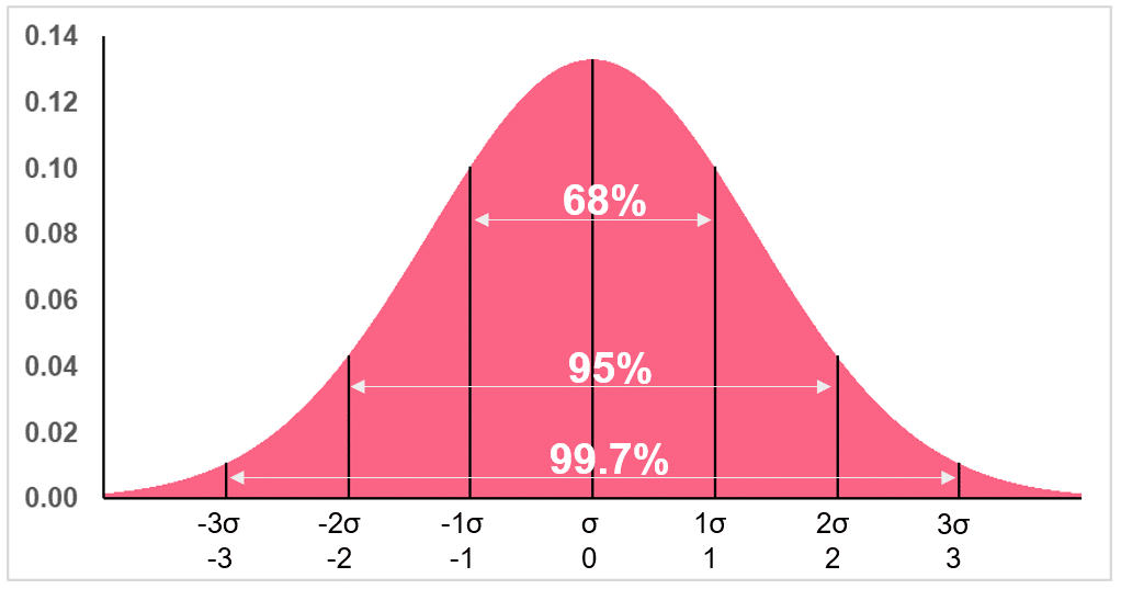
Recall the rules for interpreting z-scores. Because we are standardizing the data, the rules for a standard normal distribution apply. These interpretations are summarized below.
| Z-score | Interpretation |
| 3, -3 | Scored 3  above or below the mean, where 99.7% of the data lie between above or below the mean, where 99.7% of the data lie between |
| 2, -2 | Scored 2 above or below the mean, where 95% of the data lie between |
| 1, -1 | Scored 1 above or below the mean, where 68% of the data lie between |
| 0 | Scored at the mean. |
This means that your score in the example was 3 standard deviations below the mean, where 99.7% of test takers scored. However, z-scores can also be used for an even deeper analysis with the use of z-tables.
Z-table
A use of a z-table goes hand in hand with a standard normal graph, illustrated below.
A z-table lists all the areas below, above and in between one or more z-scores, which correspond to the areas below the curve of a standard normal distribution for any given interval or point. Some properties of z-tables are listed below.
What you can do is simply take the area below or above a point, which gives you the exact percentage of the distribution that falls above or below the curve. While you can do this by following the rules of calculus, this would be too computationally demanding - which is where the z-table comes in.
While we may be able to interpret a z-score such as 0.35 as a data point 0.35 away from the mean, we wouldn’t be able to give an exact percentage of the distribution that falls above or below that point.
The z-score in itself can be helpful when it is equal to or close to one of the major points on the standard normal distribution, such as 0 or negative 1, 2 and 3. This is because we have a rule of thumb - the 68-95-99.7% rule - that makes our analysis easy. What happens, however, when we attain a z-score of 0.35? Or one equal to 2.78?
To think about how a z-table and a standard normal distribution relate to each other, it can be helpful but not necessary to understand some basic calculus concepts. What the distribution shows is simply the probability of each and every standard deviation occurring. While the major points are emphasized, such as positive and negative 3, 2, 1 and 0, think about how many values occur between 0 and 1.
| Property | Explanation |
| The maximum value of a z-table is 1 | In probability theory, there are two extremes: something can be between either 0% likely or 100% likely. This translates to all probability distributions, where the area under the curve of the standard normal distribution is equal to 1, because 100% of the values can only occur under this curve. |
| Right Tail Z-Table | There are two types of z-tables, where the right tail z-table lists the percentage of the distribution that falls to the right of a given (which is why it’s called a right tail) |
| Left Tail Z-Table | This z-table lists the percentage of the distribution that falls to the left of a given |
A snippet of the left tail z-table can be seen in the table below.
| Z | 0.00 | 0.01 | 0.02 |
| 0.0 | 0.5000 | 0.5040 | 0.5080 |
| 0.1 | 0.5398 | 0.5438 | 0.5478 |
| 0.2 | 0.5793 | 0.5832 | 0.5871 |
If we had a z-score equal to 0.113, you would take the value in the tenth’s place, which is 0.1, and find that on the left most column. Then, you would take the rounded value of the hundredth’s place, which is 0.01, and find that on the top column. The intersection of these points is the percentage of values that fall to the left of 0.113.
This is broken down further below using the score of 74.904, the mean of 74, and the standard deviation of 8.
\[
z_{i} = \dfrac{74.904 - 74}{8} = 0.113
\]

Because this is a left tail distribution, we would interpret this number in the following manner:
- There is about 54% of the distribution that is located below 74.904
Problem 1
You took a national exam which will, unfortunately, play a major role in your college admissions. You have an estimate of how many points you scored and also the mean and standard deviation from the tests last year. Assuming the mean and SD are the same for this year’s test takers, what percentage of test-takers scored above you given that:
- Your score is 1900
- The mean score was 1600
- The SD was 140
Look up your z-value in the left tail z-table below.
| Z | 0 | 0.01 | 0.02 | 0.03 | 0.04 | 0.05 |
| 2 | 0.97725 | 0.97778 | 0.97831 | 0.97882 | 0.97932 | 0.97982 |
| 2.1 | 0.98214 | 0.98257 | 0.98300 | 0.98341 | 0.98382 | 0.98422 |
| 2.2 | 0.98610 | 0.98645 | 0.98679 | 0.98713 | 0.98745 | 0.98778 |
Solution Problem 1
In order to find the percentage of test-takers scoring above 1900, we would normally need a right-tail z-table. However, we also know that the area under the probability distribution is 1, or 100%. This means that the right-tail probability is simply:
\[
P_{right} = 1 - P_{left}
\]
Finding the z-score, we get,
\[
z_{i} = \dfrac{(1900-1600)}{140} = 2.14
\]
Looking at the table above, we can see that the left-tail probability is 0.98382, which is about 98.4%. This means that 98.4% of people scored below 1900. Naturally, the people that scored above 1900 would be,
\[
P_{right} = 1 - 0.98382 = 0.01618
\]
Which is about 1.6%.
Did you like this article? Rate it!


Can you help me answer my activities