Chapters


The Interquartile Range
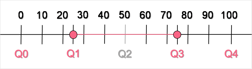
In the previous sections, you were introduced to quartiles and the interquartile range, otherwise known as the IQR. To briefly recap, the interquartile range is defined as the distance between the first and third quartiles, which contains both the median and 50% of the data. Recall the image below, used as an example illustration of the IQR.
While the IQR has many applications, including ones tied to the discussion on outliers explained further on in this section, what is important to note is how the measures of central tendency play into the IQR. This is easiest to see when looking at data plotted on a boxplot.

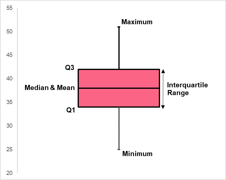
Boxplots can be an effective way of displaying the IQR because they can display many measures of central tendency and variability. The mean and median can be seen in both plots, where the boxplot on the left shows a boxplot where the mean is greater than the median and the boxplot on the right shows a distribution where the median and mean are equal.
The distribution, defined as how the variables are spread out, is best interpreted by the IQR. The boxplot on the left shows a boxplot where the first quartile is closer to the median than the third quartile. The boxplot on the right, on the other hand, shows a distribution where the median and mean are equidistant from both quartiles 1 and 3.
These differences in where the measures lie on the boxplot are due to differences in distributions. Where the distribution on the right is indicative of a normal distribution, the one on the left signals a skewed distribution. We’ll go more into more detail on distributions later. For now, you can find a recap of the measures of central tendency and variability you can observe from boxplots in the table below.
| Measure | Location on Boxplot | Interpretation |
| Mean | Typically located above or below the mean and within the IQR, although there are exceptions | The average of the data |
| Median | Located at quartile 2 | Half the data fall above and below this point (the 50% mark) |
| Minimum | Located at Q0 | The lowest value of the data set |
| Maximum | Located at Q4 | The highest value of the data set |
| Interquartile Range | Between Q1 and Q3 | Holds 50% of the data, the median and information about the centre 50% of the data set |
Outliers
If you’ve never heard of outliers in a mathematical or statistics setting, you’re bound to have heard it used in other disciplines. This is due mainly because of the fact that the definition of outliers is broad and can therefore be applied to situations beyond mathematics.
An outlier is defined as a point that diverges from the typical pattern. In other words, an outlier is different from the rest of the data set.
Influential Observation
It’s easy to confuse outliers with influential observations. However, it can be easier to separate the two by thinking of outliers as a measure belonging mainly to descriptive statistics while influential observations are typically used when utilizing inferential statistics.
An influential observation is a data point or points that have an impact on the slope of a regression line. Reserving the details of regression for our guide on inferential statistics, you can get a basic understanding of the difference between these two statistical concepts from the images below.

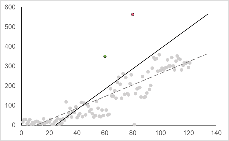
As you can see, the regression line on the left is not affected by the inclusion of the red point, whereas on the right, we can see that the regression line changes significantly with the inclusion of the pink point. This suggests the red point is an outlier and the pink point is an influential observation.
How to Identify Outliers
In statistics, there are many different ways to identify whether or not a point is an outlier. There are two basic methods you can employ to identify an outlier, which are summarized in the table below.
| Method | Description | Example |
| Standard Deviation Method | If the data has a normal distribution, we can use the 68-95-99.7 rule to determine outliers. This means we can arbitrarily set limits, typically 3  and above, to identify outliers. and above, to identify outliers. | If we set it at 3 , this means that any point 3 away from the mean and beyond can be considered outliers. |
| Interquartile Range Method | If the data doesn’t have a normal distribution, we can use the IQR as a benchmark for outliers as it contains 50% of the data. Typically, the limits are, again, arbitrarily set at IQR *  away from the 25th and 75th quartiles, where is typically set at 1.5. away from the 25th and 75th quartiles, where is typically set at 1.5. | If Q3 is 10 and Q1 is 3, the IQR would be 10 - 3 = 7. Then, the lower limit and upper limit for the data set would be 7*1.5 = 10.5. This means that any point below 3-10.5 = -7.5 and above 10+10.5 = 20.5 could be considered an outlier. |
Practice Problem 1
Calculate the following descriptive statistics from the data given in the table below:
- Median
- Mean
- Interquartile Range
| Observation | Value |
| 1 | 5 |
| 2 | 16 |
| 3 | 24 |
| 4 | 28 |
| 5 | 30 |
| 6 | 31 |
| 7 | 32 |
| 8 | 35 |
| 9 | 95 |
Problem 2
You are trying to decide whether or not you have an outlier in your data set. Use the standard deviation method in order to determine if there are any outliers in your data, given in the data table below.
| Observation | Value |
| 1 | 4 |
| 2 | 6 |
| 3 | 3 |
| 4 | 9 |
| 5 | 60 |
| Mean | 16.4 |
| Standard Deviation | 24.5 |
Problem 3
Interpret the chart below.

Solution Problem 1
| Observation | Value |
| 1 | 5 |
| 2 | 16 |
| 3 | 24 |
| 4 | 28 |
| 5 | 30 |
| 6 | 31 |
| 7 | 32 |
| 8 | 35 |
| 9 | 95 |
| Total | 296 |
The mean is calculated as,
\[
\bar{x} = \dfrac{296}{9} = 32.9
\]
The median is the midpoint of the data set. Because our data is already ordered form least to greatest, we simply need to find the middle value. In this case, it is the 5th observation, which has a value of 30.
The interquartile range is found by splitting the data into fourths. Doing this gives us the following quartiles:
- Q0 = 5
- Q1 = 24
- Q2 = 30
- Q3 = 32
- Q4 = 95
Next, the IQR can be calculated as,
\[
IQR = Q3 - Q1 = 32-24 = 8
\]
Solution Problem 2
Find the step-by-step solution below.
| Observation | Value |
| 1 | 4 |
| 2 | 6 |
| 3 | 3 |
| 4 | 9 |
| 5 | 60 |
| Mean | 16.4 |
| Standard Deviation | 24.5 |
Using the standard deviation method to identify an outlier can be done by standardizing the data point. We suspect the fifth observation may be an outlier.
\[
z_{i} = \dfrac{60-16.4}{24.5} = 1.78
\]
This means that the 60 is about 1.8 away from the mean. While this is still well within the 3 normally used for finding outliers in the standard deviation method, you may want to consider setting the limit at a lower since the sample size is small.
Solution Problem 3
| Quartile | Interpretation |
| Q0 | The minimum, located at 0 |
| Q1 | 25% of the data is below 35 |
| Q2 | 50% of the data is above and below 50 |
| Q3 | 75% of the data is below 65 |
| Q4 | The maximum, located at 100 |
Did you like this article? Rate it!


Can you help me answer my activities