Chapters


What are Polynomial Functions?
| Linear function |  | Two monomials |
| Quadratic function | 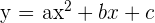 | Three monomials |
| Cubic function | 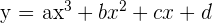 | Four monomials |
You may have noticed the term ‘monomial.’ A monomial is the basic building block of polynomials. Let’s take a look at the different types of monomials.
 |  |  |  |
| One variable | One constant | One variable times one constant | One constant times two or more variables |
When we combine monomials, we can form the polynomial equations form before.
As long as we have one or more monomials, we have a polynomial equation. However, polynomial equations with one, two and three monomials also have special names. We know monomial, and in the image above we can see: binomial and trinomial.
Rational Functions
Rational functions are defined as two polynomial functions divided by each other. In other words, we have one polynomial function in the numerator and one polynomial function in the denominator.

Remember that a polynomial is any function with one or more monomials. This means that technically, all polynomial functions are also rational functions. This is because any polynomial function can be re-written to be divided by 1. Take a look at the image below.

| Numerator |  | Binomial |
| Denominator | 1 | Monomial |
When we are given a rational function, the first thing we need to do is simplify it. Simplification means that we are grouping all variables together and all constants together as much as possible. Let’s take a simple example.

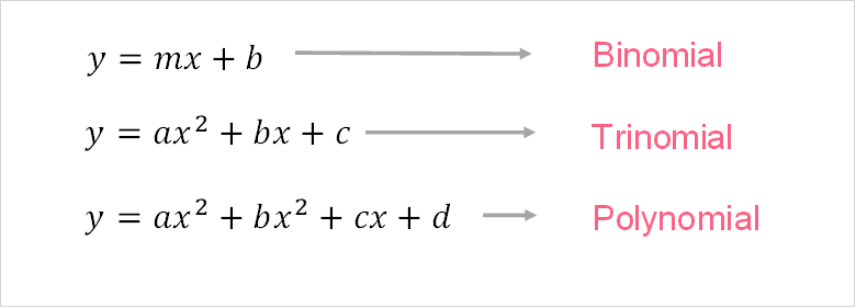
If you remember, when we have a fraction, we can transform it into the following.

This can often be the first step in simplifying rational functions. Let’s apply it to our example.
Now that we have simplified the rational function, it is a lot easier to graph.
| x | y |
| 1 | 7 |
| 2 | 5 |
| ... | |
| 10 | 3.4 |
Here are some other simplifications rules that can help you:
Common Polynomials
Now that we have gone through all the building blocks of rational functions, we can begin to discuss how to graph rational functions. Since the goal of simplifying rational functions is to reduce them to a polynomial, we will start with graphing the most common polynomials.
Linear Polynomial
As mentioned, the linear polynomial is the easiest polynomial to graph. We only have four elements in a linear polynomial.
| y | Output | Dependent variable |
| m | Slope | The rate of change |
| x | Input | Independent variable |
| b | y-intercept | Value of function if x = 0 |
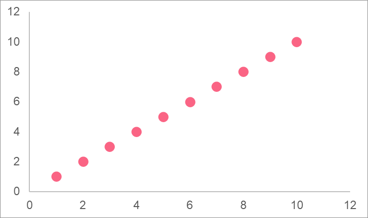
To graph a linear polynomial, simply plug in values of x in order to get the resulting y value. No matter what equation or x values you choose, a linear polynomial will always result in a straight line.
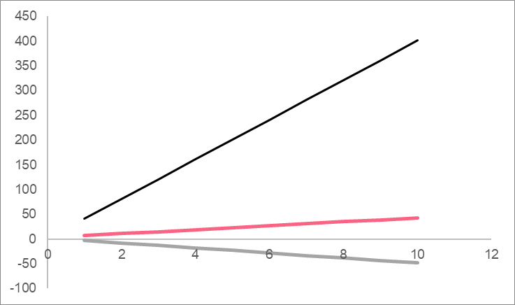
| A | B | C |
| y = 4x + 3 | y = -5x + 2 | y = 40x+1 |
Quadratic
A quadratic equation has a degree of two. Degrees in polynomial functions mean the highest value of power in the equation.
| Degree 2 | |
| Degree 3 | |
| Degree 4 |  |
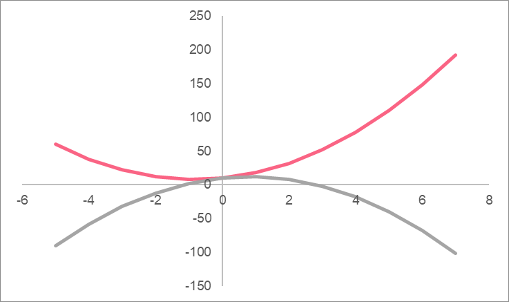
In order to graph a quadratic equation, you should simply plug in values of x and plot the resulting y. The shape of a quadratic equation will always be a parabola. One easy trick to remember is:
| Negative sign in front of a |  | Parabola shape is  |
| Positive sign in front of a | | Parabola shape is  |
Cubic
A cubic function has a degree of 3. Just like the other polynomials we’ve talked about, graphing a cubic function involves picking values for x and graphing the resulting coordinates. A cubic function will always result in an ‘S’ shape.
Just like with a quadratic function, depending on the sign in front of the ‘a’ term, this ‘S’ shape can either be normal or backwards. Take a look at the examples below.
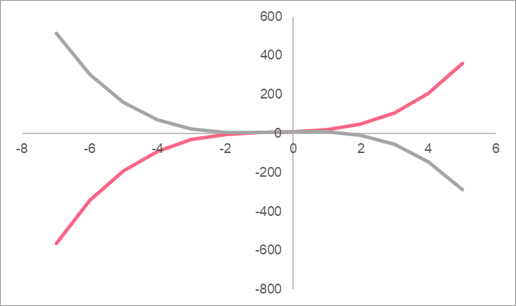
| A | B |
| |
Graphing Simple Rational Functions
Now that we have a good grasp on all the components that go into graphing rational functions, let’s start by graphing simple rational functions.

There are two different polynomials in the denominator and numerator:
| A | Binomial | Linear function |
| B | Monomial | Linear function |
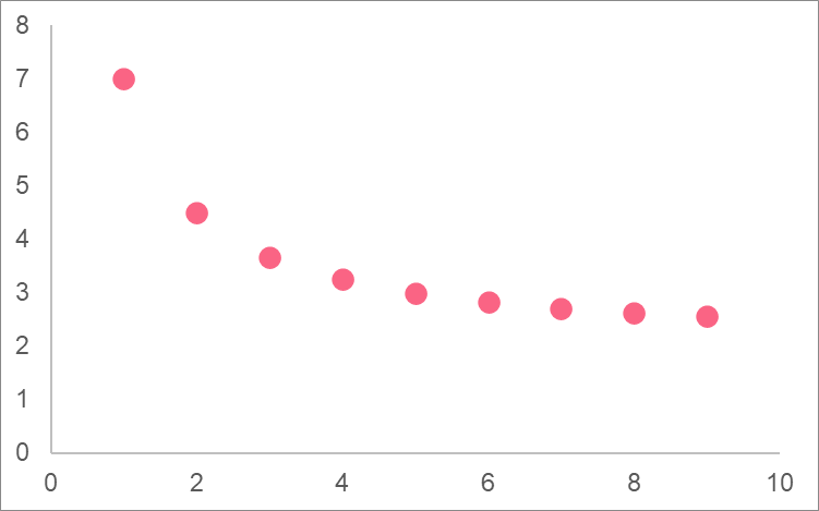
There are two ways we can do this, simply plug in values for x and plot the coordinates:
| x | y |
| 1.0 | 7.0 |
| 2.0 | 4.5 |
| 3.0 | 3.7 |
Or simplify the equation first:

Either way, we get the following:
Graphing Complex Rational Functions
When you’re graphing more complex rational functions, you can follow either of the two processes we mentioned above. Let’s take an example:

The polynomials here are:
| A | Trinomial | Quadratic function |
| B | Binomial | Linear |
| C | Binomial | Linear |
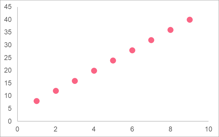
We can plug in values of x:
| x | y |
| 1 | 8 |
| 2 | 12 |
| ... | ... |
However, this can take too long with more complex rational functions. So instead, we prefer to simplify first.
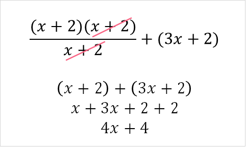
Step-by-step Example
Let’s graph the following rational function:

First, in order to simplify this rational function, we first look for any patterns. Let’s take the two elements of the equation separately. Starting with the first one, we have one trinomial and one binomial. Let’s factor the first one:

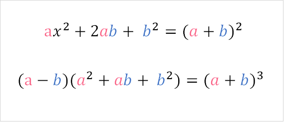
The binomial follows a perfect square pattern. This means we can factor it in the same way.
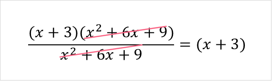
Now, we can simplify the terms.

Next, we simplify the second rational function.

Putting it all together, we get the following.

Did you like this article? Rate it!


