Chapters


Introduction to Linear Programming
It is an optimization method for a linear objective function and a system of linear inequalities or equations. The linear inequalities or equations are known as constraints. The quantity which needs to be maximized or minimized (optimized) is reflected by the objective function. The fundamental objective of the linear programming model is to look for the values of the variables that optimize (maximize or minimize) the objective function.
We know that in linear programming, we subject linear functions to multiple constraints. These constraints can be written in the form of linear inequality or linear equations. This method plays a fundamental role in finding optimal resource utilization. The word "linear" in linear programming depicts the relationship between different variables. It means that the variables have a linear relationship between them. The word "programming" in linear programming shows that the optimal solution is selected from different alternatives.
We assume the following things while solving the linear programming problems:
- The constraints are expressed in the quantitative values
- There is a linear relationship between the objective function and the constraints
- The objective function which is also a linear function needs optimization
Features of Linear Programming
The linear programming problem has the following five features:
Constraints
These are the limitations set on the main objective function. These limitations must be represented in the mathematical form.
Objective function
This function is expressed as a linear function and it describes the quantity that needs optimization.
Linearity
There is a linear relationship between the variables of the function.
Non-negativity
The value of the variable should be zero or non-negative.
Parts of Linear Programming
The primary parts of a linear programming problem are given below:
- Objective function
- Decision variables
- Data
- Constraints
Why we Need Linear Programming?
The applications of linear programming are widespread in many areas. It is especially used in mathematics, telecommunication, logistics, economics, business, and manufacturing fields. The main benefits of using linear programming are given below:
- It provides valuable insights to the business problems as it helps in finding the optimal solution for any situation.
- In engineering, it resolves design and manufacturing issues and facilitates in achieving optimization of shapes.
- In manufacturing, it helps to maximize profits.
- In the energy sector, it facilitates optimizing the electrical power system
- In the transportation and logistics industries, it helps in achieving time and cost efficiency.
In the next section, we will discuss the steps involved in solving linear programming problems.
Steps to Solve a Linear Programming Problem
We should follow the following steps while solving a linear programming problem graphically.
Step 1 - Identify the decision variables
The first step is to discern the decision variables which control the behavior of the objective function. Objective function is a function that requires optimization.
Step 2 - Write the objective function
The decision variables that you have just selected should be employed to jot down an algebraic expression that shows the quantity we are trying to optimize. In other words, we can say that the objective function is a linear equation that is comprised of decision variables.
Step 3 - Identify Set of Constraints
Constraints are the limitations in the form of equations or inequalities on the decision variables. Remember that all the decision variables are non-negative; i.e. they are either positive or zero.
Step 4 - Choose the method for solving the linear programming problem
Multiple techniques can be used to solve a linear programming problem. These techniques include:
- Simplex method
- Solving the problem using R
- Solving the problem by employing the graphical method
- Solving the problem using an open solver
In this article, we will specifically discuss how to solve linear programming problems using a graphical method.
Step 5 - Construct the graph
After you have selected the graphical method for solving the linear programming problem, you should construct the graph and plot the constraints lines.
Step 6 - Identify the feasible region
This region of the graph satisfies all the constraints in the problem. Selecting any point in the feasible region yields a valid solution for the objective function.
Step 7 - Find the optimum point
Any point in the feasible region that gives the maximum or minimum value of the objective function represents the optimal solution.
Now, that you know what are the steps involved in solving a linear programming problem, we will proceed to solve an example using the steps above.
Example
A bakery manufacturers two kinds of cookies, chocolate chip, and caramel. The bakery forecasts the demand for at least 80 caramel and 120 chocolate chip cookies daily. Due to the limited ingredients and employees, the bakery can manufacture at most 120 caramel cookies and 140 chocolate chip cookies daily. To be profitable the bakery must sell at least 240 cookies daily.
Each chocolate chip cookie sold results in a profit of \ 0.88 profit.
a) How many chocolate chip and caramel cookies should be made daily to maximize the profit?
b) Compute the maximum revenue that can be generated in a day?
Solution
Part a
Follow the following steps to solve the above problem.
Step 1 - Identify the decision variables
Suppose:
Number of caramel cookies sold daily = x
Number of chocolate chip cookies sold daily = y
Step 2 - Write the Objective Function
Since each chocolate chip cookie yields the profit of \ 0.88, therefore we will write the objective function as:
 , where x and y are non negative
Step 3 - Identify Set of Constraints
It is mentioned in the problem that the demand forecast of caramel cookies is at least 80 and the bakery cannot produce more than 120 caramel cookies. Therefore, we will write this constraint as:

It is also mentioned that the expected demand for the chocolate chip cookies is at least 120 and the bakery can produce no more than 140 cookies. Therefore, the second constraint is:

 is subjected to the following constraints:
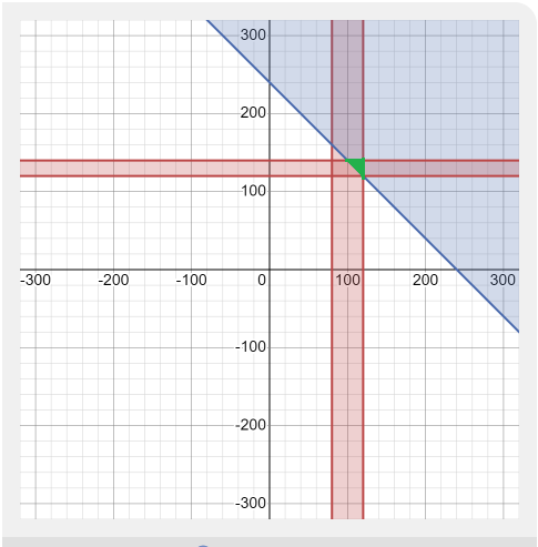
The green area of the graph is the feasibility region.
Step 7 - Find the Optimum point
Now, we will test the vertices of the feasibility region to determine the optimal solution. The vertices are:
(120, 120) , (100, 140), (120, 140)
(120, 120) P = 0.88 (120) + 0.75 (120) = \ 193
193
(120, 140) P = 0.88 (120) + 0.75 (140) = \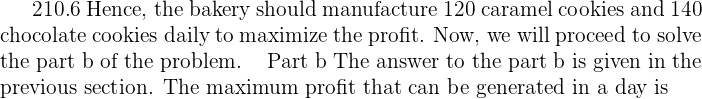 210.6.
Did you like this article? Rate it!


An agricultural Research institute suggested to a farmer to spread out at least 4800kg of a special phosphate fertilizer and not less than 7200kg of a special nitrogen fertilizer to raise productivity of crops in his fields. There are two sources for obtaining these: Mixture A and B, both of these are available in bags weighting 100 kg each and they cost sh 40 and sh24 respectively. Mixture A contains phosphate and nitrogen equivalent of 20 kg and 80 kg respectively, while mixture B contains these ingredients equivalent of 50 kg each.
Required: Write this as a linear programming problem and determine how many bags of each type the farmer should buy in order to obtain the required fertilizer at a minimum cost
Very good
Please help to do under this question
A company produces two types of TVs, one of which is black and white, the
other colour. The company has the resources to make at most 200 sets a week. Creating a black
and white set includes Birr 2700 and Birr 3600 to create a colored set. The business should
spend no more than Birr 648,000 a week producing TV sets. If it benefits from Birr 525 per set
of black and white and Birr 675 per set of colours.
Construct the linear programing model.
How many sets of black/white and colored sets it should produce in order to get
maximum profit using
Graphical Method and Simplex Method
A company manufacture two types of product A1 and A2. Each product using milling and drilling machine. The process time per unit of A1 on the milling is 10 hours and the drilling is 8 hours, the process time per unit of A2 on the milling is 15 minute and on the drilling is 10 hours, the maximum number of hours available per week on the drilling and milling machine are 80 hours and 60 hours respectively also the profit per selling of A1 and A2 are 25 naira and 35 naira respectively. Formulate a LP model to determine the production volume of each of the product such that the total profit is maximized
so this equestion of linear programming what have a solution
A linear programming problem
Please help to do this qutions,
Ethio Manufacturing, a renowned company in Ethiopia, specializes in
producing two types of products: Product A and Product B, with the primary
objective of maximizing its total profit. Each unit of Product A yields a profit
of 5 Birr, and each unit of Product B yields a profit of 4 Birr.
The company is
constrained by limited resources in two vital departments: Department A, with 60 hours of available production time, where producing one unit of
Product A consumes 3 hours and one unit of Product B consumes 2 hours;
and Department B, with 72 hours of available production time, where
producing one unit of Product A takes 4 hours and one unit of Product B
takes 3 hours. Questions
1. Formulate the Linear Programming Problem (LPP):
2.Graphically analyze the LPP to determine the optimal production quantities
of Product A and Product B that maximize Ethio Manufacturing’s profit. Identify the coordinates of the optimal solution point.
3. Apply the simplex method to find the optimal solution for Ethio
Manufacturing’s LPP. Present the initial tableau, pivot steps, and the final
solution. Explain each step in the simplex method.
4. Determine the dual problem for Ethio Manufacturing’s LPP and present
the dual problem’s objective function and constraints.
5a. Discuss the changes in objective-function coefficients (cj) of the optimal basic feasible solution
5b. Discuss the effect of discrete change in the avaliabilty of resources from
[60, 72 ]T to [70, 50]T
Hi pls hw d u obtain d constraints in for truck type B in exercise 1