Chapters


What is Regression?
| Hours Spent on Phone | Hours Spent Outside |
| 2 | 0.5 |
| 1 | 0.6 |
| 5 | 0.2 |
| 3 | 0.4 |
With descriptive statistics, which measures the centre and spread of the data, we could calculate the mean number of hours spent on their phone or outside. We could also calculate the variance in the data or plot the number of hours spent on their phone with a bar chart.
While descriptive statistics are very powerful, inferential statistics can help us predict what is not included in our dataset. Regression analysis is one of the tools of inferential statistics, which models the linear relationship between two or more variables. Take a look at the image below, which you’ll be able to interpret by the end of this guide.

Simple Linear Regression
Simple linear regression is a form of linear regression in which there is only one independent and one dependent variable. To understand these variables, take a look at the image below.
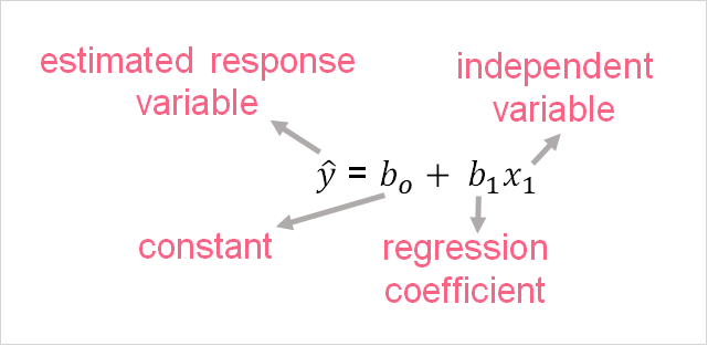
This is the sample SLR equation, which closely follows the equation of a line, which can be seen below.

As you can see, the SLR equation is composed of four main components. These components are explained in the table below.
| Component | Definition | Interpretation |
| Y | Response variable | The variable that increases or decreases in response to changes in x |
| X | Explanatory variable | The variable that describes the variation in y |
| Bo | Constant | The value of y if x was zero |
| B1 | Slope | The amount of increase or decrease (if positive or negative) in y following a 1 unit change in x |
SLR Interpretation
In order to understand how to interpret and SLR model, you should know that besides the four elements mentioned above, there are typically two more elements given in a regression model, summarized below.
| Component | Definition | Interpretation |
| R-squared | Proportion of variance of the response variable explained by the explanatory variables | A high R-squared indicates the regression model is good at explaining the variance in y |
| Standard error of regression | The standard error between the data points and the predicted values | A low SE of the regression means that the data points and predicted values are close together |
Problem 1
You are interested in studying the relationship between income level and energy consumption. In order to do this, you are given a data set that includes the variables income and energy consumption. The income variable is in thousands of dollars while the energy consumption variable are in megawatt hours, or MWh.
Calculate the covariance and correlation coefficient of these variables. Using this information, interpret the graph of both variables which is given below.
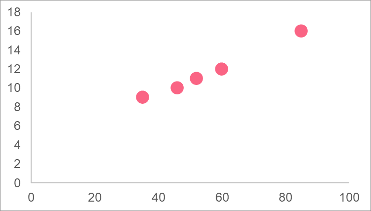
| Income | Energy Consumption |
| 35 | 9 |
| 46 | 10 |
| 52 | 11 |
| 60 | 12 |
| 85 | 16 |
Solution to Problem 1
In this problem, you were asked to calculate the correlation coefficient and then interpret the variables in the graph using this information. To calculate the correlation coefficient, you first have to calculate the mean of both x and y. Next, you subtract this value from each observation and plug the results into the formula.
| Income | Energy Consumption |  |  |  |  |  |
| 35 | 9 | -21 | -3 | 53.56 | 424.36 | 6.76 |
| 46 | 10 | -10 | -2 | 15.36 | 92.16 | 2.56 |
| 52 | 11 | -4 | -1 | 2.16 | 12.96 | 0.36 |
| 60 | 12 | 4 | 0 | 1.76 | 19.36 | 0.16 |
| 85 | 16 | 29 | 4 | 129.36 | 864.36 | 19.36 |
| Mean = 56 | Mean = 12 | Total | 202 | 1413 | 29 |
\[
r(x,y) = \dfrac{202}{\sqrt{1413*29}} = 0.995
\]
Problem 2
In the previous problem, you were asked to explore the relationship between the two variables of energy consumption and income level using the covariance and correlation coefficient. Now, you want to see if there is another factor in determining energy consumption. You are given a data set that, for the same energy consumption observations, has data on the average temperature in that region.
Given the following graph of the two variables, calculate the correlation coefficient of the two variables and compare it to the previous two variables. In other words, find out if income level and energy consumption are more strongly or weakly correlated than average temperature and energy consumption.
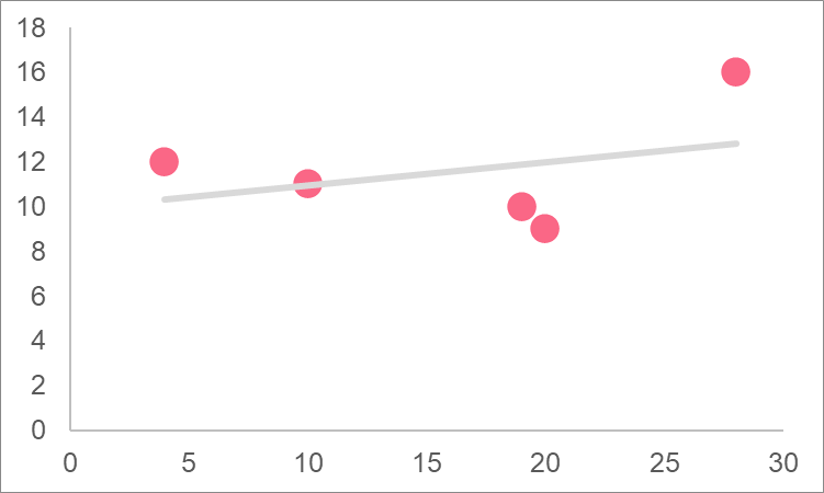
| Average Temperature | Energy Consumption |
| 20 | 9 |
| 19 | 10 |
| 10 | 11 |
| 4 | 12 |
| 28 | 16 |
Solution to Problem 2
In order to compare the two variables, we need to find the correlation between average temperature and energy consumption.
| Average Temperature | Energy Consumption | | | | | |
| 20 | 9 | 4 | -3 | -9.88 | 14.44 | 6.76 |
| 19 | 10 | 3 | -2 | -4.48 | 7.84 | 2.56 |
| 10 | 11 | -6 | -1 | 3.72 | 38.44 | 0.36 |
| 4 | 12 | -12 | 0 | -4.88 | 148.84 | 0.16 |
| 28 | 16 | 12 | 4 | 51.92 | 139.24 | 19.36 |
| Mean = 16 | Mean = 12 | Total | 36 | 349 | 29 |
\[
r(x,y) = \dfrac{36}{\sqrt{349*29}} = 0.361
\]
Income and energy consumption are more highly correlated than average temperature and energy consumption.
Problem 3
You have now determined which variables are more strongly correlated. In order to be able to use this information, you need to use the data to model energy consumption. That is, you need to build an SLR model with the data that you have. Recall that there are two main elements you need to calculate in order to build an SLR model: the constant and the regression coefficient. You can find these formulas below.

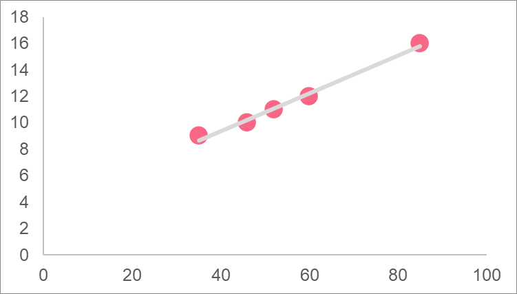
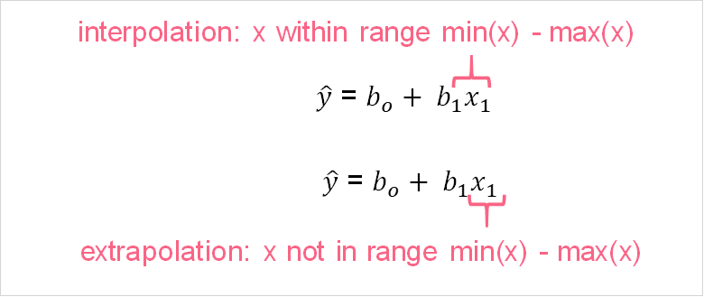
Find the SLR model using the data of the most strongly correlated variables. Next, perform an interpolation and extrapolation using any values. Recall that interpolation is when you predict y using an x variable that is already included in the range of your data set. Extrapolation, on the other hand, is when you predict a y using an x that is outside the range of your data. The picture below should give a clearer idea.
Solution to Problem 3
In order to build a regression model, we must find the values for b_{o} and b_{1}. Recall the information we already calculated.
| 56 |
| 12 |
| 202 |
| 1413 |
| 29 |
 |  |
=  = 0.14 = 0.14 |
 |  |
=  = 3.6 = 3.6 |
Did you like this article? Rate it!


