Chapters


Correlation
| Correlation Coefficient | Interpretation |
| -1 | Perfect negative linear relationship |
| 0 | No linear relationship |
| 1 | Perfect positive linear relationship |
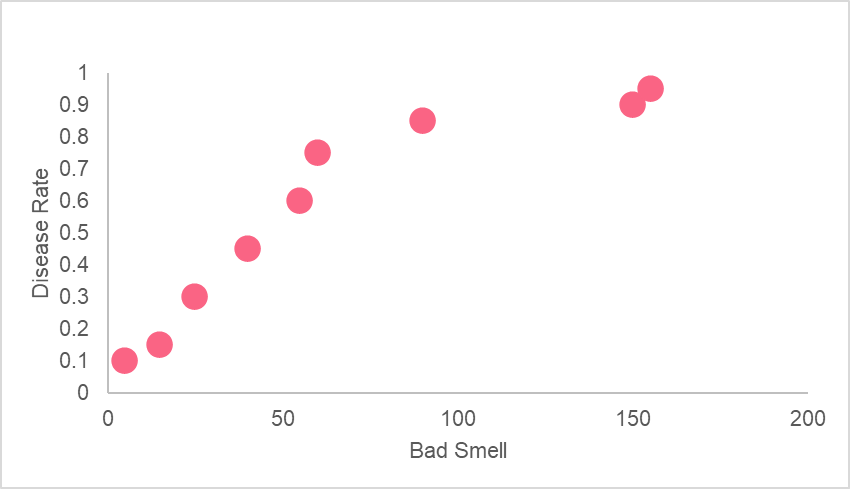
In our example, this means that sour two variables, ad smell and disease, have a strong positive linear relationship. However, this doesn’t mean that bad smells cause disease. A high correlation between the two indicates the fact that they share a common, underlying relationship with another factor. In this case, this happens to be germs.
Statistical Models
A statistical model is a mathematical model that strives to make predictions or generalizations about a population using a sample from that population. A regression model is an example of a statistical mode. However, this doesn’t mean that regression models are the only statistical models.
On the contrary, statistical models are many and diverse. Take a look at the table below to get an idea of the other types of statistical models out there.
| Statistical Model | Description |
| Regression Analysis | Estimates relationships between one response variable and one or more explanatory variables |
| Cluster Analysis | Groups observations into groups so that groups are homogenous and different groups are more heterogeneous |
| Discriminant Analysis | Classifies data into groups and is used to choose relevant variables (dimension reduction) |
SLR
As you can probably guess, simple linear regression, or SLR, is a type of regression model used in regression analysis. In SLR, only one response variable and one explanatory variable are examined. Take a look at the equation and example below.

As you can see in the example above, there is only one response variable - demand - and one explanatory variable - price. This is a classic example of the applications of statistical models in the field of economics.
Here, we can see the four main components of SLR, which are summarized in the table below.
| Y | Demand | Response variable |
| Bo | (123) | Constant, the value if x is zero |
| B1 | (23) | Regression coefficient, the amount that y increases with 1 unit increases in x |
| x | Price | The observed demand of an individual |
As you can see, these four components make up the regression model. The SLR model can be used to predict the demand given x, the price. For example, if the price for t-shirts increases by 10 pounds, the owner of the store would be able to predict the demand for t-shirts.
SLR Interpretation
The interpretation of an SLR model can be quite simple, given that you understand what the output means. The output of a regression model is typically given by some statistical software, be it Excel, R, Python or more.
You don’t typically have to calculate this by hand, although you can. After all, these concepts were invented before there were even calculators. Most statistics courses will require you to calculate these statistics by hand before showing you how to find them using statistical software. This is only to help you get a deeper understanding of what each metric means.
However, if you will be analysing any two variables, it is recommended that you use some sort of software or program. That way, you can spend more time interpreting your results rather than memorizing how to calculate each and every statistic.
R squared Interpretation
The R-squared value is typically seen as the most important component of a standard output. The image below shows what this regression model output looks like in the program R.
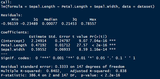
As you can see, there are typically two types of r-squared values that you see in a regression model output. The only difference between the two is that the R-squared adjusted adjusts the R-squared to take into account the number of independent variables in you have in your regression model.
In order to interpret the R-squared value, you should know that it reflects the proportion of the variance in the response variable that is explained by the independent variable. Knowing this definition will help you remember why independent variables are often called explanatory variables.
| R-Squared | Interpretation |
| > 0.90 | Something may be wrong with your model, as high R-squared values can be an indication of things like multicollinearity |
| 0.9 > R2 < 0.4 | The explanatory variables explain much of the variance in the response variable |
| R2 < 0.4 | The explanatory variables provide a very weak, or non-existent, explanation for the response variable |
Above, you can see how people generally interpret the R-squared value. However, there are a couple more statistics to take into account before deciding if your model is good or not.
F-statistic and P-Value Interpretation
The F-statistic in the regression output goes hand in hand with it’s corresponding p-value. Take a look at the image below, which shows the F-statistic and p-value for our regression model output.
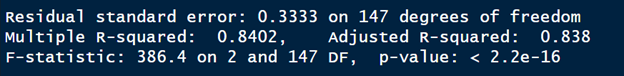
Keep in mind that any time you see some letter and statistic, it usually indicates there’s some sort of hypothesis test going on. For example, F-statistic is the ratio between the explained and unexplained variation in your model. The higher the F-statistic, the better your parameters are at explaining the response variable. The p-value is interpreted as below.
| P-value | Interpretation |
| P-value < 0.05 | Reject the null hypothesis, Ho, which states that the model explains no variability in the data |
| P-value > 0.05 | Fail to reject the hull hypothesis, Ho |
Coefficients
The coefficients are interpreted as the amount of increase in your y variable given a 1 unit increase in you x variable, all other variables held constant. For example, if you have a regression coefficient of 0.3, y would increase by 0.3 with an increase of 1 unit of x.
Problem 1
You have the following regression model, whose elements have been broken down into those we’ve discussed in this section.
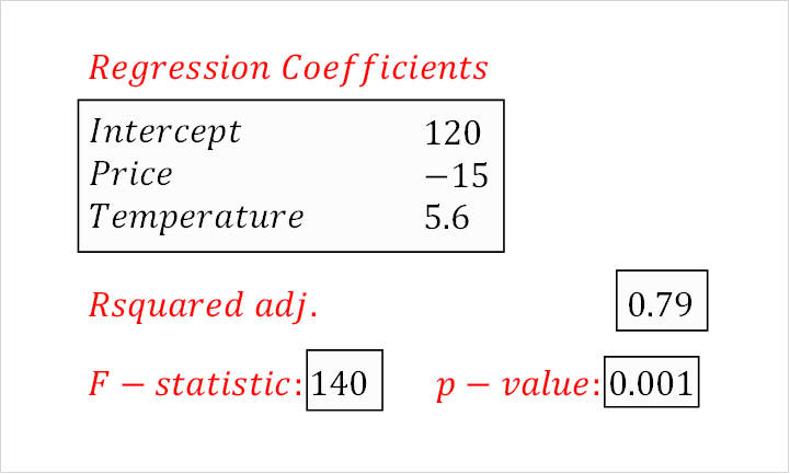
Demand for ice cream is modelled here by the price and the temperature outside. Interpret each element of the output above.
Solution to Problem 1
Here, you were asked to interpret the given output. First, recall that the adjusted R-squared value is the explained variation of your model. Here, our model accounts for 79% of the variation in demand for ice cream.
Looking at the f-statistic and p-value, we can see that with a p-value less than 0.05, our parameters do a good job of explaining the variation in ice cream. All other variables held constant, an increase of 1 dollar in price would decrease ice cream demand by 15. On the other hand, an increase of 1 degree in temperature increases demand for ice cream by 5.6.
Did you like this article? Rate it!


