Solution to Problem of Regression 7

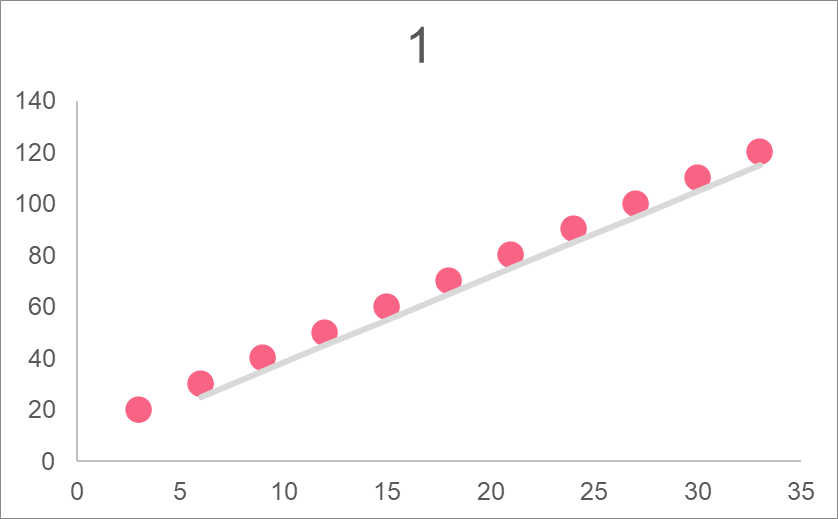
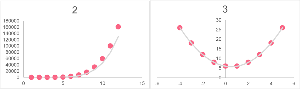
Graph	Relationship	Equation	Formula
1	Parabolic	Quadratic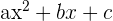
2	Exponential	Exponential growth
3	Linear	Line

We can model data by finding the best line to represent the data. This is why regression is used, because it can be used to model the data that is available and predict the future.

Single Linear Regression

Simple linear regression is a type of regression. Simple linear regression, or SLR, involves only one dependent and one independent variable. Notice that the equation for SLR follows closely to that of a line. The image below illustrates where these variables are located in a regression equation.

The difference between the response and explanatory variables are summarized in the table below.

Notation	Variable	Definition
y,	Response, dependent	Variable we want to predict
X, x	Explanatory, Independent	Variable used to predict response variable

As you may notice, there are two formulas for SLR. The difference between the two are explained in the table below.

Equation	Variables	Type	Data used
1	y, , X,	Population SLR	Data on the entire population is used. The true population parameters are calculated.
2	, b, x	Sample SLR	Data using a sample from the population is used. True population parameters are estimated.

Multiple Linear Regression

Multiple linear regression, or MLR, is quite similar in definition to SLR. The difference between the two is that in an MLR model, more than one independent variable is used to estimate the dependent variable. Take a look at the equations below.

The two equations represent the same as the SLR equations, the top equation is the population MLR equation and the bottom equation is the sample MLR equation. The table below defined what each element in the formulas mean.

	Element	Description	Definition
1	y	Response variable	The variable we’re trying to predict
2	and	Constant	The value of y when all x’s are zero
3	and b’s	Regression coefficients	The amount y increases or decreases given a 1 unit change in x
4	x’s	Independent variables	The variable used to predict y
5		Error	The random error, the part of y that isn’t explained by x

MLR Estimators

There are many different approaches you can use to estimate a MLR model. The most common approach is to use any program that has the capability of calculating an MLR model given a data set. Another rare approach is to calculate an MLR model by hand. While this is not convenient and can lead to errors of calculation, it can be helpful for someone trying to understand the concepts behind regression.

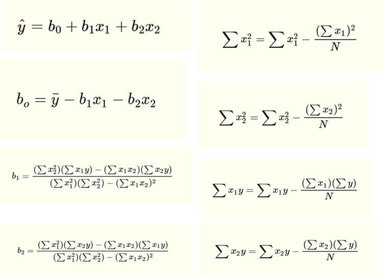
Estimating MLR regression coefficients is a bit more difficult than for SLR coefficients. However, the general idea is the same. The picture below shows the equations.

MLR Interpretation

When it comes to interpreting an MLR model, the intuition is the same as for a SLR model. However, because there are more explanatory variables, there are a few more things you should take into account. Check out the table below in order to get a better idea on how to interpret these variables given a MLR model with two independent variables.

Element	Interpretation
	Value of y when all independent variables are zero
	Value that y increases or decreases by given a change of 1 unit in x when b_{2} variables held constant
	Value that y increases or decreases by given a change of 1 unit in x when b_{1} variables held constant

Variable Transformations

Transforming variables are a common operation that is completed before a MLR model is run. The reason why some variables are transformed can be:

• To have the variable follow a better distribution
• To create a new variable
• To improve the appearance in visualizations

These are the most common reasons why variables are transformed. Some common transformations to perform on a variable are:

• Logarithm
• Square
• Square root

Interpretation with Transformed Variables

Interpreting a MLR model with transformed variables depends on the type of transformation performed. Typically, square or square root transformations are easier because the number is still on the same scale. Logarithmic transformations are a bit more complex because they involve a logged scale. The table below summarizes the interpretation of models using logarithm transformed values.

Type	Model	Interpretation of Regression Coefficients
Log-log	y and x are log transformed	An 1% increase of x will lead to a ()% in y
Linear-log	x is log transformed	An 1 unit increase of x will lead to an increase of (/100) units in y
Log-linear	y is log transformed	An 1 unit increase in x will lead to an increase of (100*())% in y

Problem 1

You are tasked with interpreting the following MLR model.

Using what you know about how regression estimators are calculated, write a short summary describing the model.

Solution to Problem 1

When temperature and ad expenditure are both zero, there will still be 100 tickets sold. As the temperature increases by 1 degree, ticket sales increase by 1.3 tickets all other variables held constant. As ad expenditure increases by 100 pounds, ticket sales increase by 5.4 tickets.

Problem 2

Salary is a variable that typically has a right-skewed distribution. This is because most people tend to make around the same amount of money, with some people making extreme amounts of money. Because of this, a log transformation has been performed on salary. Interpret the following model.

Solution to Problem 2

The constant is not interpretable here, as salary and vacation days will never be zero. Every 1 day increase in vacation days increases the happiness score by 2 points. An 1 unit increase of salary will lead to an increase of 0.04 points in happiness score.