Chapters


What is Linear Regression?
Have you ever wondered how statistics are calculated? For example, according to Statistica, in 2017 to 2018, people in the UK drove, on average, about 16,000 km. But how exactly do statisticians arrive at such a number?
Statistics, and maths in general, have been the source of much contention these days. In the face of alternative facts, understanding how statistics are calculated is an extremely important skill. Statistical analysis revolves around one main concept: we cannot access all data all the time. This is why statistical analyses are produced, in order to be able to estimate certain phenomena, such as how many kilometres people drive on average in the UK every year.


The image above is a visual representation of what a sample is along with some of the questions one must consider when taking a sample. The table below shows it’s definition, as well as what it means in our specific example.
| Population | All things included in the phenomena we want to study | All of the cars driven in the UK |
| Sample | Subset of the population | A sample of 1,000 cars driven in the UK |
What multiple linear regression, otherwise known as MLR, attempts to do is build a model that uses explanatory variables to predict one response variable. The data used in this MLR, for the majority of the time, comes from a sample. This means that the MLR model that we calculate is only an estimate of the MLR model that exists for the entire population.
Take a moment to refresh your memory on what measurements are called and mean for both the population and sample.
| Population | The entire group of things, ideas, or people we want to study | Population parameters are measurements from the population | Population MLR model |
| Sample | Subset of the population | Sample statistics are measurements from the sample that strive to estimate the true population values | Sample MLR model that estimates the population MLR |
Applications of Linear Regression
The applications of MLR are vast. Take a look at the MLR equations below that correspond to the population and the sample.

As you can see, the four main components of an MLR model are present. These include:
- The response variable
- The explanatory variables
- The parameters of the model
- The constant
An example of an MLR model in real life can be seen in the image below.

In this example, we take the current pandemic into account. This model strives to predict the amount of covid cases in a given region given the population, number of hospitals, and average flights per day in that region. In this example, the four main components can be broken down like the table below.
| Response variable | Number of covid cases |
| Explanatory variables | Population, number of hospitals, average flights per day |
| Parameters of the model | Beta values, which will be predicted using a data set |
| The constant | The Bo value, which is the constant in the model |
Transformed Variables
In the majority of cases, the data from our sample has moderately to highly skewed variables. Skewed variable is a variable whose distribution is heavier on one tail. Take the image below as an example.

This distribution plot shows the average annual income of a sample of adults. As we would expect, there are a lot less people that earn higher annual salaries. However, if you are trying to predict the which factors go into determining annual salaries, it’s not variable you can just scrap.
This is where the idea of transforming variables comes into play. If you want to use a variable but it has a highly skewed distribution, like the one above, you can transform it so that it’s distribution will have a more normal distribution. You should think about transforming your variable if it is highly skewed.
| Skewness Coefficient | Interpretation |
| > 1 or < -1 | Highly skewed |
| 1 > skew > 0.5 or - 1 < skew < - 0.5 | Moderately skewed |
| 0.5 > skew > - 0.5 | Approximately symmetric |
As you can see, if the skewness coefficient is greater than 1 or less than -1, then you should think about transforming your variable. The common types of transformations are summarized below.
| Logarithm | Take the log of the variable |
| Cube root | Take the cube root of the variable |
| Square root | Take the square root of the variable |
| Square | Square the variable |
Taking the log of the above values yields the following distribution. As you can see, our variable is no longer skewed and can be used without problems in our MLR.

Transformed Variables Interpretation
As we discussed, highly skewed variables are generally transformed. This is because skewed variables can lead to biased statistics. For example, recall our previous example which used annual income. Because the original variable is highly right skewed, this means that the majority of the data are located around lower salary values with only a few observations located around higher salary values.
If we were to take the mean of this highly skewed data, you can imagine it would give us a higher value than what is actually the most common salary in our dataset. The higher salary values act as inflators, pushing the mean up because of their magnitude. Now imagine this effect in a regression!
Take a look at the table below to see how log transformed variables are interpreted for common types of linear regression models.
| Type | Interpretation of Regression Coefficients |
| Log-log | An 1% increase of x will lead to a (coefficient)% in y |
| Linear-log | An 1 unit increase of x will lead to an increase of (coefficient/100) units in y |
| Log-linear | An 1 unit increase in x will lead to an increase of (100*(coefficient))% in y |
Transformed Variables Example
Let’s take a look at an example to put the above interpretations into perspective. The following model plots the association between the area and population.
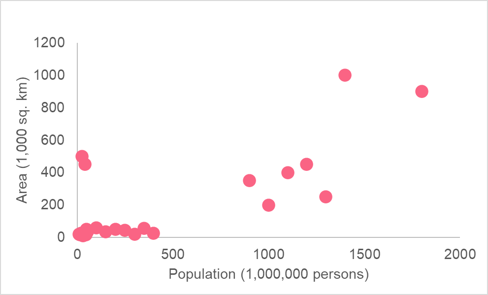
As you can see, the area is in 1,000 square kilometres while the population is in millions. From this graph, it is unclear what relationship there is, if any. This is because there is an extreme difference in range between where most of the values for population and area are when compared to the more extreme values.
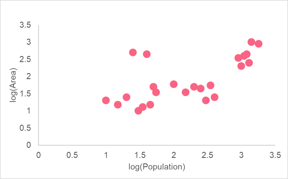
As you can see, taking the logarithm of both variables allows us to see a more clearly defined relationship for both variables. This is because a logarithmic scale is not linear - meaning, the difference between 1 and 2 versus 6 and 7 are not the same distance. Moving one unit on the log scale means multiplying by 10 each time.
Problem 1
A model has been run based off of the previous example. The following summarizes the output of each regression element.
| y | Log of area |
| bo | The constant in the model is 3,000 |
| b1 | The regression coefficient for population is 9.8 |
| x | Log of population |
Interpret the results of the regression
Solution Problem 1
Using the information given in this section, we can interpret the regression in the following way.
| 3,000 | Here, the constant can be interpreted as the area of land given that the population is zero |
| 9.8 | An 1% increase in population will lead to a 9.8% in area |
Did you like this article? Rate it!


