Chapters


Probability
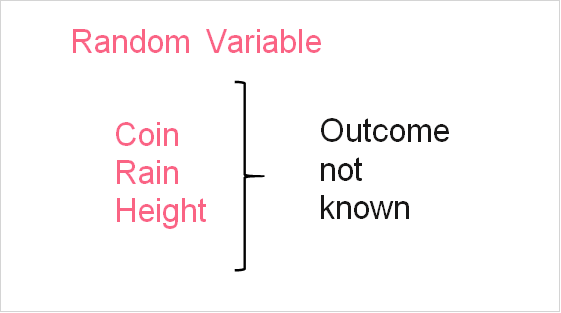
A random variable is a variable whose outcome is unknown. A die toss is a classic example of a random variable: the outcome is unknown until the moment the die is tossed.

All possible outcomes of the random variable makeup it’s sample space, whose notation you can see in the image above. An event, on the other hand, is simply one or more outcomes in the sample space.


Probability, then, can be defined as the likelihood of an event occurring. The simplest formula for probability is located below.
\[
Probability = \frac{# \; of \; possible \; outcomes \; (Event)}{All \; possible \; outcomes \; (Sample Space)}
\]
Probability Distribution
A probability distribution is a visualization of all possible outcomes of a random variable along with the probability of each value occurring. Let’s revisit the die roll example: say you want to know the probability of having a sum of 2 when rolling 2 dice.
| 1 | 2 | 3 | 4 | 5 | 6 | |
| 1 | (1,1) | (1,2) | (1,3) | (1,4) | (1,5) | (1,6) |
| 2 | (2,1) | (2,2) | (2,3) | (2,4) | (2,5) | (2,6) |
| 3 | (3,1) | (3,2) | (3,3) | (3,4) | (3,5) | (3,6) |
| 4 | (4,1) | (4,2) | (4,3) | (4,4) | (4,5) | (4,6) |
| 5 | (5,1) | (5,2) | (5,3) | (5,4) | (5,5) | (5,6) |
| 6 | (6,1) | (6,2) | (6,3) | (6,4) | (6,5) | (6,6) |
Next, we figure out the probability of each sum of dice. Notice that the minimum sum we have is 2, because 1+1=2, and the maximum sum is 12. Each diagonal has the same sum. For example, take a look at the first two diagonals.

This makes it easy for us to come up with the probabilities of each sum occurring, which is the probability distribution.
| Sum | Probability (Fraction) | Probability (Decimal) |
| 2 | 1/36 | 0.028 |
| 3 | 2/36 | 0.056 |
| 4 | 3/36 | 0.083 |
| 5 | 4/36 | 0.111 |
| 6 | 5/36 | 0.139 |
| 7 | 6/36 | 0.167 |
| 8 | 5/36 | 0.139 |
| 9 | 4/36 | 0.111 |
| 10 | 3/36 | 0.083 |
| 11 | 2/36 | 0.056 |
| 12 | 1/36 | 0.028 |
This gives us the following probability distribution.

Standard Normal Distribution
We looked at a simple probability distribution for rolling 2 dice - however, what if we wanted to know the probability distribution of another random variable. For example, the distribution for a coin toss or the distribution for the amount of cars on the highway? Every random variable has its own probability distribution. While there are many different kinds, we can focus on a standard normal distribution.
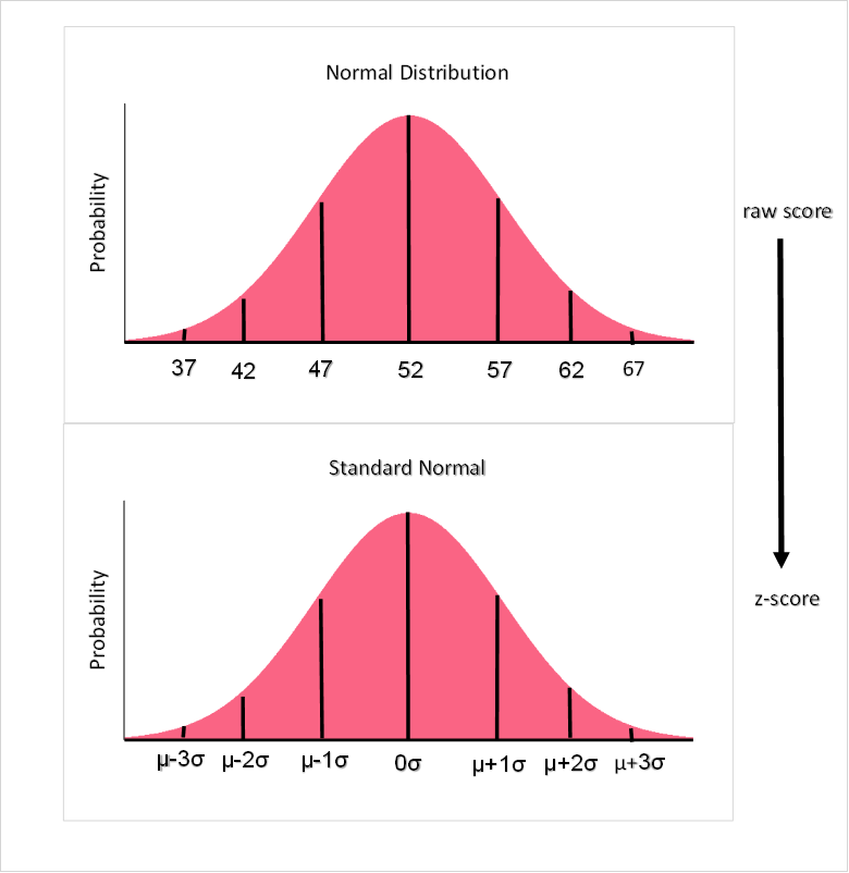
A normally distributed variable is one whose probability distribution is shaped like a bell, which is why they are also known as “bell-shaped” distributions. Dice rolls, when rolled enough times, actually have normal distributions.
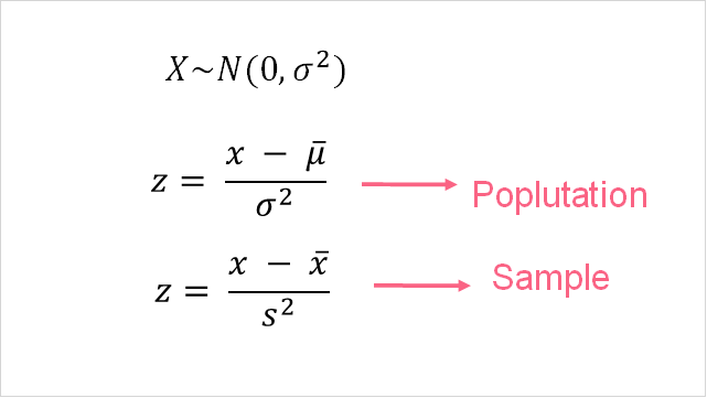
The only difference between a normal and standard normal distribution is the scale of the numbers. While a normal distribution has the values of the x-axis as raw scores, the standard normal distribution has it’s values in z-scores.
Binomial Distribution
Binomial distributions are those whose random variables have only two outcomes. Some examples are listed in the table below.
| Example | Outcomes |
| Result of an interview | Success or Failure |
| Coin toss | Heads or Tails |
| Exam score | Pass or Fail |
The parameters for a binomial distribution are below.

The elements of the probability formula are explained below.
| Element | Description |
| n | Number of trials (called Bernoulli trials) |
| k | Number of successes in n trails |
| p | Probability of success |
| q | Probability of failure (q = 1-p) |
Poisson Distribution
A poisson distribution, on the other hand, is a distribution that deals with time. Some examples of random variables with poisson distributions are given below.
| Example | Example Outcome |
| Number of calls at a call centre per hour | 15 calls per hour |
| Number of hours a lightbulb will function | 100 hours |
| Number of clients at a store during the day | 200 clients per day |
To calculate the probability of a poisson distribution, we use the characteristics of the parameters, listed below.
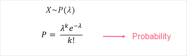
| Element | Description |
 | Mean rate (mean # occurrences per interval) |
| e | Natural |
| k | Probability of success |
Problem 1
A call centre for an amusement park has been experiencing many complaints from customers who are unhappy about long waiting times. The call centre has a policy that states that if you wait for more than half an hour, you will get a gift card to the amusement park.
Wanting to improve call times, the call centre wants to know how likely it is that 32 customers will call in 4 hours given that the average number of calls per hour is 5. First, state which distribution you would use.
Solution 1
In order to solve this, first you should understand what type of distribution we’re dealing with here. The distribution we would use to solve this is a Poisson distribution. The reason for this is that we’re dealing with intervals of time.
Next, we need to outline what each parameter is, shown in the picture below.

Problem 2
Next, continuing from problem 1, you want to calculate the probability of 32 people calling in four hours given that the average amount of calls per hour is 5. Solve this scenario.
Solution 2
While it may seem there is more than one way to solve this, there is only one way. Because we want to compare the amount of people calling in 4 hours and not per hour, we can simply multiply 5 by 4. This is because each interval of 1 hour has an average of 5 calls.
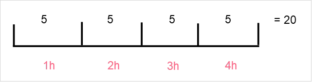
\[
P(32) = \frac{20^{32} e^{-20}}{32!} = 0.0034 = 0.34%
\]
We cannot solve this problem by dividing the number of people in 4 hours by 4 hours. In other words, find how many people are calling per hour if the total is 32 in 4 hours. This gives us a different probability.
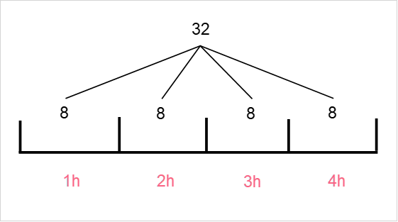
\[
P(8) = \frac{5^{8} e^{-5}}{8!} = 0.065 = 6.5%
\]
Did you like this article? Rate it!


Using facebook account,conduct a survey on the number of sport related activities your friends are involvedin.construct a probability distribution andbcompute the mean variance and standard deviation.indicate the number of your friends you surveyed
this page has a lot of advantage, those student who are going to be statitian
I’m a junior high school,500 students were randomly selected.240 liked ice cream,200 liked milk tea and 180 liked both ice cream and milktea
A box of Ping pong balls has many different colors in it. There is a 22% chance of getting a blue colored ball. What is the probability that exactly 6 balls are blue out of 15?
Where is the answer??
A box of Ping pong balls has many different colors in it. There is a 22% chance of getting a blue colored ball. What is the probability that exactly 6 balls are blue out of 15?
ere is a 60% chance that a final years student would throw a party before leaving school ,taken over 50 student from a total of 150 .calculate for the mean and the variance
There are 4 white balls and 30 blue balls in the basket. If you draw 7 balls from the basket without replacement, what is the probability that exactly 4 of the balls are white?