Chapters


Probability
| Definition | Notation | Example | |
| Probability | The likelihood of some event occurring | P(event) | P(A) -> Probability of event A occurring |
| Random Variable | A variable whose outcome is unknown until the random experiment has been run | X,Y,Z,M, etc. | X -> a coin flip |
The reason why these two concepts are linked is because we typically calculate the probability of one or several outcomes of a random variable. Random variables are different from traditional variables in that you don’t know what the outcome is until the moment the event actually happens.
The outcome of a coin flip, for example, cannot be known until the coin lands on either side. This is the reason we use probability to model it’s outcomes.
Probability Distribution
A probability distribution is a visualization that plots possible outcomes on the x-axis and each of the probabilities associated with those outcomes on the y-axis. Let’s continue with the coin flip example to illustrate this. Let’s see the probability of getting heads for 3 coin flips.
| Coin Flips | Events | Sample Space | Possibilities | Number Equivalents | Probability of Heads |
| 0 | P(H) or P(T) | S = {H,T} | 0 | 0 | P(H) = 0 |
| 1 | P(H) or P(T) | S = {H,T} | H T | 1 0 | P(0) = 1/2 P(1) = 1/2 |
| 2 | P(H) or P(T) | S = {H,T} | HH TT HT TH | 2 0 1 1 | P(0) = 1/4 P(1) = 2/4 P(2) = 1/4 |
| 3 | P(H) or P(T) | S = {H,T} | HHH TTT HHT HTH HTT THH THT TTH | 3 0 2 2 1 2 1 1 | P(0) = 1/8 P(1) = 3/8 P(2) = 3/8 P(3) = 1/8 |
As you can see, when we start with only 1 coin flip, it is easy to calculate the probabilities for each outcome because there are only two possibilities. As you increase the amount of flips you do, the possible outcomes also increase. We can graph each distribution on a graph.

Types of Distributions
There are many different kinds of distributions. The example that we gave above is one example of a very common distribution known as a binomial distribution. The table below lists the three common distributions, their properties and when they should be used.
| Distribution | Notation | Definition | Used When | Example |
| Binomial/Bernoulli | X ~ B(n,p) | Distribution with parameters n and p | There’s only two outcomes (heads/tails, pass/not pass, success/failure, etc.) | Coin toss |
| Normal/ Standard Normal | X ~ N( , , ) ) | Distribution with parameters and | The random variable X has a normal distribution | IQ scores |
| Poisson | X ~ P( ) ) | Distribution with parameter | The random variable is related with time | Number of hours a lightbulb works |
Normal Distribution Properties
A normal distribution, which can also be transformed into a standard normal distribution, is used in many scenarios in probability. A normal distribution is usually called a “bell-shaped curve,” because the probability distribution is shaped like a bell. Take IQ scores of the population, for example.
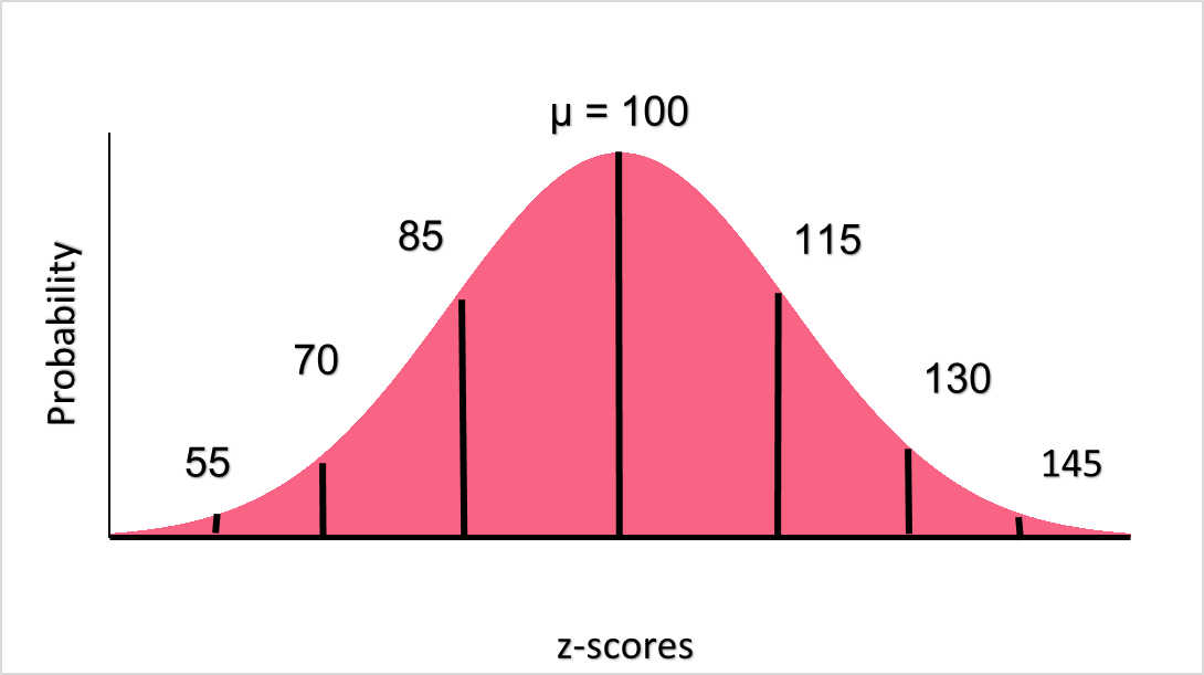
As you can see, IQ scores have a bell-shaped distribution. While visual confirmation is normally enough, we can also conduct statistical tests to make sure the distribution is normal or not. The IQ scores plotted above are in raw form. We can transform each IQ score by standardizing them, which we do by plugging in the raw score into the z-score formula below.

This gives us the same distribution - only now, each IQ score is in terms of how many standard deviations away from the mean it is.

This gives us some special properties of a normal distribution, which we can see in the table below.
| Standard Deviation | Percentage | Description |
| -1 , +1 | 68% | 68% of the data fall in the interval between -1 and +1 standard deviations. This means 65% of the population are within 1 standard deviation from the mean |
| -2, +2 | 95% | 95% of the data fall within 2 sd from the mean |
| -3, +3 | 99.7% | 99.7% of the data fall within 3 sd from the mean. After this point, it will be rare. |
Right Tail Probability
We can calculate the probability of a given value occurring through the z-score formula because the properties of the normal distribution are always the same, regardless of what the mean or standard deviation are. Contrast this to all the work we did to calculate the probabilities of a coin toss by hand!
Right tail probabilities are when we want to know the probability of a value equal to or above a value. The image below illustrates.
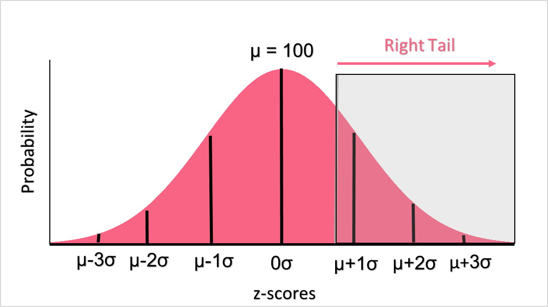
Once you find the z-score, you simply find it on the right-tail z-table. The probability in this table will be compared to the significance level you choose, which will tell you whether to reject or accept your hypothesis.
Left Tail Probability
In contrast, when we want to know the probability of a value equal to or less than a value, this would be a left tail probability. The image below shows what a left-tail probability looks like on a normal distribution.
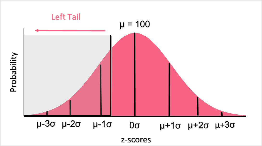
While you can find the left-tail z-table for this, you can also just use 1 minus the right tail probability.
Probability for an Interval
When you want to know the probability that a value will be in between two values, this is called an interval probability. Take a look at the image below.
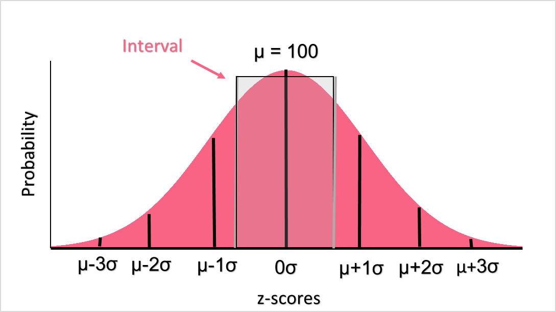
While it may seem complicated to be able to distinguish between these three types of probabilities, the information is summarised below for your ease.
| Type | Notation | Example | Z-table | Probability |
| Right Tail | P(x > a) | P(X > 140) | Right tail, or (1- ) ) |  , 1- , 1- |
| Left Tail | P(x < b) | P(X < 110) | Left tail, or (1-) | , |
| Interval | P(a < x < b) | P(120 < X < 135) | Either |  - - , ,
|
 -
-
Step-by-Step Example
The population average IQ score is 100 with a standard deviation of 15 points. We calculate the following probabilities, given an alpha of 0.05.
| IQ Score | Type | Notation | Z-score |
| Above 110 | Right | P(x>110) |  = 0.67 = 0.67 |
| Below 80 | Left | P(x<80) |  = -1.33 = -1.33 |
| Between 85 and 115 | Interval | P(85<x<115) |  = -1, = -1,  - 1 - 1 |
Next, we look up the z-score in the z-table for each.
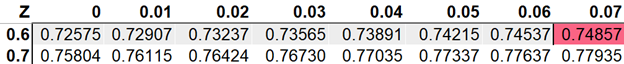
The p-value for a score of 110 is about 0.75, which is above our alpha of 0.05. This means this value is likely, or we ‘retain’ the null hypothesis if we were running a hypothesis test.
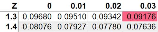
The p-value for a score of 80 is 0.092, which is above our alpha of 0.05. As you can see, both 110 and 80 are either below 1 standard deviation away from 100 or just a bit above 1 SD away.
To get the interval, we can look at the picture below.
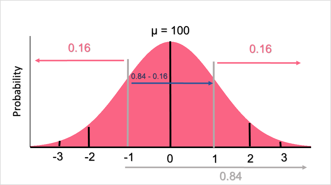
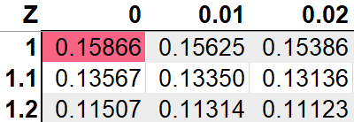
First we get the left tail probability of 0.15866.

Next we get the right tail probability of 0.84134. Because the standard deviation is 1 and -1, we can see that the left tail probability at -1 is 0.15866, while the right tail probability at the same point would be 0.84134. To get the portion in the middle, we simply:
\[
p-value = 0.8134-0.15866 = 0.68268
\]
Which we could have guessed, as the rules of a normal distribution dictate that between -1 and 1 is 68% of the population.
Did you like this article? Rate it!


Using facebook account,conduct a survey on the number of sport related activities your friends are involvedin.construct a probability distribution andbcompute the mean variance and standard deviation.indicate the number of your friends you surveyed
this page has a lot of advantage, those student who are going to be statitian
I’m a junior high school,500 students were randomly selected.240 liked ice cream,200 liked milk tea and 180 liked both ice cream and milktea
A box of Ping pong balls has many different colors in it. There is a 22% chance of getting a blue colored ball. What is the probability that exactly 6 balls are blue out of 15?
Where is the answer??
A box of Ping pong balls has many different colors in it. There is a 22% chance of getting a blue colored ball. What is the probability that exactly 6 balls are blue out of 15?
ere is a 60% chance that a final years student would throw a party before leaving school ,taken over 50 student from a total of 150 .calculate for the mean and the variance
There are 4 white balls and 30 blue balls in the basket. If you draw 7 balls from the basket without replacement, what is the probability that exactly 4 of the balls are white?