Chapters


Hypothesis Definition
| Variable A | Variable B | Hypothesis |
| Rain | Tourists | More rain leads to less tourists in the city |
| Phone battery | Temperature | Extreme temperatures lead to lower battery life |
| Air quality | Disease | An increase in air quality leads to a decrease in diseases |
As you can see, hypotheses are quite simple. In fact, you have probably made a hypothesis today!
While hypotheses are used in many areas, such as psychology or biology, they can also be used in statistics. Hypotheses in statistics can help us suggest explanations for probabilistic events. Take a look at the table below, comparing the general definition of a hypothesis with that of a statistical hypothesis.
| Hypothesis | Statistical Hypothesis | |
| Definition | A suggested explanation for an event | An assumption about a parameter that can be tested with a data set |
| Example | Votes increase with increased media pressure | The mean number of votes is different between two populations: one with no media influence, one with media influence |
Hypothesis Testing
Hypothesis testing, in general, is very simple: it means testing a hypothesis. This can be through measurements, using models, software and more. Statistical hypothesis testing, on the other hand, is one of the methods involved in inferential statistics. Take a look at the image below, describing the definition of inferential statistics.
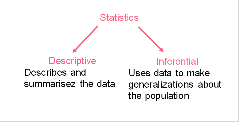
Inferential statistics try to make predictions based off of a sample dataset. In statistical hypothesis testing, there are two types of hypotheses, summarized below.
| Notation | Description | Symbols | Rejected |
| Ho | A statement about a parameter | =,<,>,etc. | When the test statistic is inside the region of rejection |
| H1, Ha | Usually the counter of Ho | =,<,>,etc. | When the test statistic is outside the region of rejection |
Probability Distribution
In order to understand what type of hypothesis test you need to run, you need to first determine the probability distribution of your variable. There are two main things we can mean when we refer to a distribution: a frequency distribution and a probability distribution. In order to understand the difference between the two, check out their definitions summarized in the table below.
| Type | Definition | Example |
| Frequency Distribution | Displays the frequency of each value of a variable occurring | The number or people in each age group from 1-100 |
| Probability Distribution | Displays the probability of each value of a variable occurring | The probability of a person being a given age from 1-100 |
As you can see, both types of distributions give us information about how the data looks like. The major difference, however, is what they tell us about the data. For example, the frequency distribution can tell us whether the variable is skewed or not.


These distributions are skewed distributions, which means that the majority of the values centre around one end of the range of values. The difference between the two distributions can be seen in the table below.
| Type | Definition | Mean | Characteristics |
| Left | Values are centred around higher values with only some values on the lower end | Lower than it would normally be, low values “deflate” the mean | Mean < Median |
| Right | Values are centred around the lower end with only some values in the higher end | Higher than it would normally be, higher values “inflate” the mean | Mean > Median |
Both the frequency and probability distributions can tell us about a variable’s spread and centre. In other words, both can give us a picture of the mean and standard deviation. However, because probability distributions display the probabilities of each value, they can be used to predict how likely certain values are. This is what makes them so useful in hypothesis testing.
Region of Rejection and Acceptance
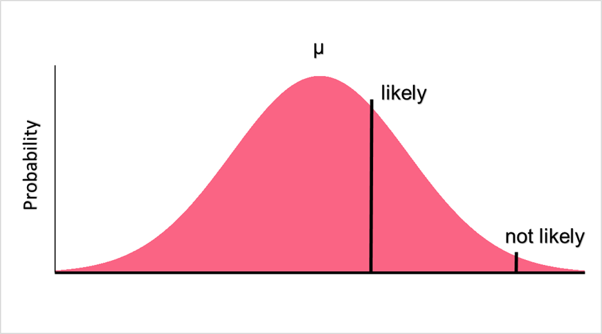
Because probability distributions can be used in hypothesis testing, we can determine how likely a certain value is to occur or not. Let’s take the following null and alternative hypotheses as an example.
| Hypothesis | Description | Explanation |
| Ho | Salary < 10,000 | The mean salary of a group of people is less than 10,000 |
| Ha | Salary > 10,000 | The mean salary of a group is more than 10,000 |
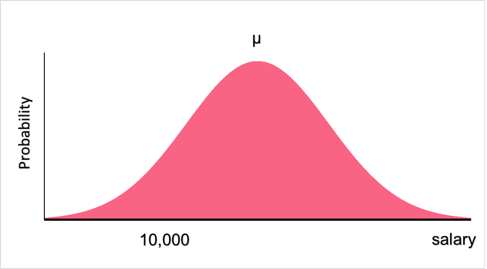
Here, the null hypothesis states that the salary of a group of people is below 10,000. However, our proposed explanation might not be true. To test this hypothesis, we use the probability distribution of salaries to see how likely a mean salary of below 10,000 would be.
Significance Level
In order to figure out whether or not we will accept a hypothesis or not, we first need to set a significance level for our hypothesis test. The significance level is the chance of committing a type 1 error, which is when we reject a null hypothesis when it is actually true. Significance levels are usually set at 0.05, 0.10 or 0.15.
Z-Score
There are two ways you can determine whether or not your value falls in the region of rejection or not. Both of these ways involve a test statistic. Test statistics are the corresponding version of a raw score on some sort of distribution. A raw score is the number you want to test, which in this case would be 10,000. Assuming that our distribution is a normal distribution, we can use the z-score as a test statistic.

Above, you can see the formulas for the population and sample z-score. This z-score will tell us how many standard deviations away our raw score is from the mean. Below, we can see the major demarcations on a normal distribution represent z-scores.
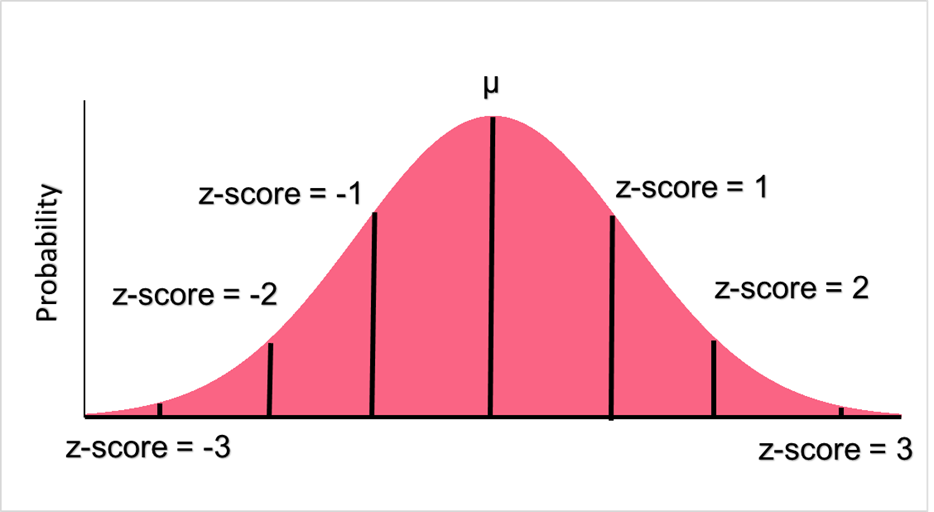
| z-score | Interpretation |
| 0 | Raw score is equal to the mean |
| 1, -1 | Raw score is 1 sd above or below the mean |
| 2, -2 | Raw score is 2 sd above or below the mean |
| 3, -3 | Raw score is 3 sd above or below the mean |
| 4, -4 | Raw score is 4 sd above or below the mean |
Z-table
Once you calculate the z-score, you find the corresponding p-value in the test statistic table, which in this case would be the z-table. A p-value is the probability of the raw score occurring in the distribution with a given mean and standard deviation. Let’s say, for example, you want to see what a p-value a z-score of 1 would be.
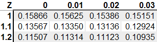
As you can see, a z-score of 1.0 would be a p-value of 0.158. At alpha equal to 0.05, the p-value would be greater than alpha and we would fail to reject the null hypothesis. Alternatively, if our alpha is set to 0.05, we can find this value on the z-table, which is 1.64. This is called a critical value - if our z-score is above this, we can also reject the null hypothesis.
Two Tailed Hypothesis Test Example
Using the example above, let’s modify the null hypothesis so that it is a two-tailed test. A two-tailed test simply means that there are two regions you have to test your hypothesis against.
| Hypothesis | Description | Explanation |
| Ho | Salary = 10,000 | The mean salary of a group of people is equal to 10,000 |
| Ha | Salary <> 10,000 | The mean salary of a group is not equal to 10,000 |
With a mean of 15,000 and a standard deviation of 4,500, the z-scores is:
\[
z-score = \dfrac{10,000 - 15,000}{4,500} = -1.11
\]
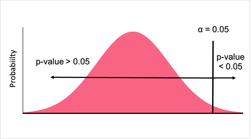
Here, the region of rejection would look like the following.
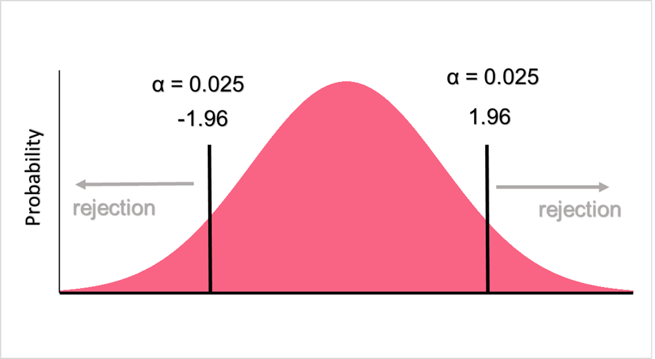
Because we’re doing a two tailed test, we have to divide alpha so that it is evenly distributed on both sides, giving us an alpha of 0.025. Next, we look up 0.025 on the z-table.
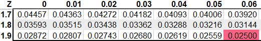
If our z-score is less than -1.96 or greater than 1.96, we reject the null hypothesis. Because our z-score is -1.11, we retain the null hypothesis that the salary is equal to 10,000.
Did you like this article? Rate it!


