Chapters


What is a Hypothesis?
In this case, you would form a hypothesis, which would be a suggested explanation for why that person is mad at you. Perhaps it’s because you made a hurtful comment or forgot something important. These explanations would be based on the history between you and that person or your characteristics. When you form a hypothesis in science or maths, the same approach is taken. First, you form your hypothesis based on previous information and then you would discover whether your hypothesis is right or wrong.
In Statistics, hypotheses are usually made with regards to the parameters or distribution of the population or sample. The image below shows the different notations for hypothesis.

Types of Hypothesis Tests
As you saw in the previous image, there are two types of hypothesis: the null and alternative hypotheses. The table below gives a definition and example of both.
| Hypothesis | Definition | Example |
| Ho | States that the population parameter is <.> or = to some value. Can also state whether a distribution is of a certain type. | The mean is < 3 |
| H1 | States that the population parameter is not <,>, or = to the same value. Can also state that a distribution is not of a certain type. | The mean is > 3 |
Notice that the alternative hypothesis is usually the opposite of the null hypothesis. In statistics, there are a massive variety of hypothesis tests. Here, we’ll focus on those relating to the parameter or distribution of the sample or population.
| Mean | Can be <,>,= to a certain value | Can be <,>,= to the population mean if want to compare to population |
| Standard Deviation | Can be <,>,= to a certain value | Can be <,>,= to the population sd if want to compare to population |
| Mean of different groups | Can be <,> to each other if want to compare between groups | Can be = if want to test if all group means are the same, fails if even just 1 is different |
Probability Distribution
In the last table, you may have noticed that hypothesis tests can depend on the distribution of a variable. However, what exactly is a distribution?
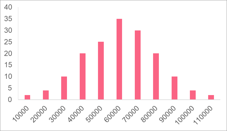
The distribution of a variable is how the variable “looks” like: it’s mean, spread, and range. In the image above, the variable salary has a skewed distribution, meaning that the majority of people have salaries to the left, while there are only a couple of people with salaries at the higher end. A histogram, like the one above, is a good way to see a variable’s distribution.
A probability distribution is similar, the only difference being that instead of telling us how often a value occurs, it tells us the probability of that value occurring. With the data from salary, we form a probability distribution. With this distribution, we can take new data regarding people’s salary and compare it to the probability distribution to see how likely those values are.
Types of Distributions
There are many different types of distributions. One that was mentioned previously were skewed distributions. In general, there are two kinds of skewed distributions, summarized below.
| Type | Definition | Characteristics |
| Left-skewed | There is a “left tail” that represents some values on the lower end and most data is located on the higher end | Mean < Median |
| Right-skewed | There is a “right tail” representing only some values on the higher end while most data is gathered on the lower end | Mean > Median |
In terms of probability distributions used in hypothesis testing, there are four major distributions to know.


The characteristics of these distributions are summarized in the table below.
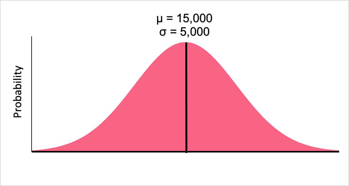
| Graph | Type | Notation | Description |
| A | Normal (Gaussian) and Standard Normal | N( , ,  ) ) | : mean
|
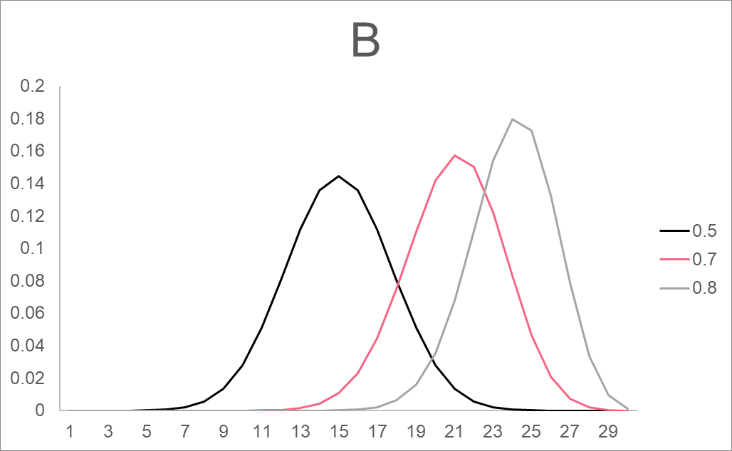
| B | Binomial | B(n, p) | n: number of trials p: probability of success |
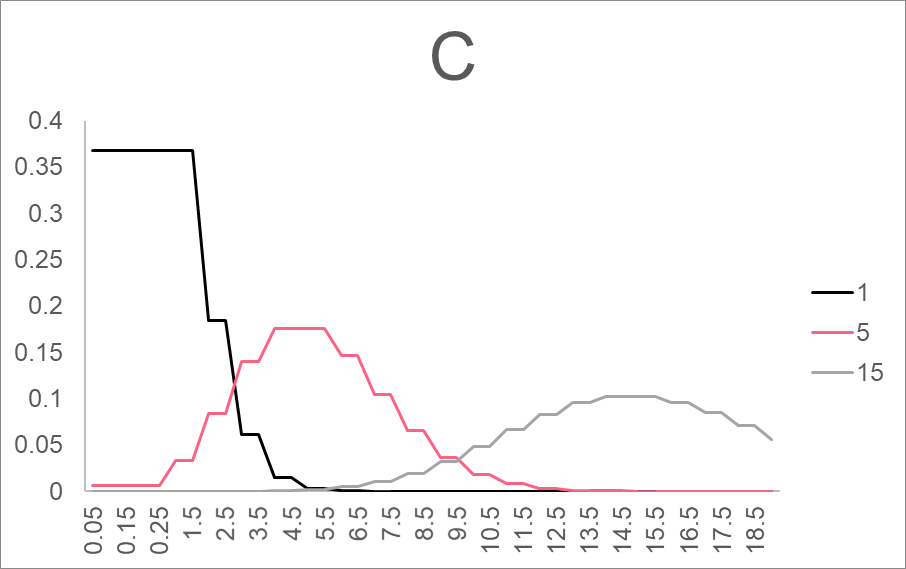
| C | Poisson | P( ) ) | : number of times something occurs per time interval (mean) |
| D | F-distribution | F(d1, d2) | d1, d2: degrees of freedom |
Significance Level
In order to test your hypotheses, you will have to chose a significance level, which is denoted by alpha,  . The significance level is generally defined as the probability of rejecting the null hypothesis when the null hypothesis is actually true. In statistics, there are two types of errors: type 1 and type 2 errors, which are defined below.
| Error | Definition |
| Type 1 | When the null hypothesis is rejected when it is actually true |
| Type 2 | When the null hypothesis is accepted when it is actually false |
The significance level can therefore be viewed as the level of risk we want in our hypothesis test of accidentally committing a type 1 error. The most common alphas are displayed below.
| Alpha | Interpretation |
| = 0.05 | 5% chance of a type 1 error |
| = 0.1 | 10% chance of a type 1 error |
| = 0.15 | 15% chance of a type 1 error |
Region of Rejection
The region of rejection is also used in decision making inside of hypothesis testing. The region of rejection is defined as the region of a probability distribution where we reject the null hypothesis if our value falls in it. This concept can be made more clear with the image below.
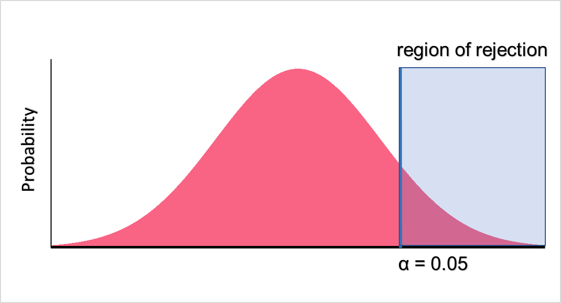
As you can see, if our value falls in the blue zone, we will reject the null hypothesis and retain the alternative hypothesis. On the other hand, if the value doesn’t fall in the blue zone, which is our region of rejection, we do not reject the null hypothesis. There are two values that are used to determine the start of the region of rejection.
| Value | Condition | Rejection |
| alpha | p-value < alpha | Reject  |
| Critical value | Test statistic > critical value | Reject |
The critical value is the value of the distribution at the point where the probability is equal to the set alpha. This can become more concrete using an example, which is done in the next sections.
Z-Score
A raw score is a value that has been unchanged. Say we have the distribution of values for wait times. If the distribution has been normalized, meaning the mean is 0 and the standard deviation is 1, we call this a standard normal distribution. See the standard normal distribution for wait times below.

We want to test the null hypothesis that a wait time is less than 5 minutes given a mean of 50 minutes and a standard deviation of 15. Here, 5 is a raw score because it is a raw data point. To be able to test this using the probabilities on a standard normal distribution, we have to convert it into a test statistic. The test statistic for a standard normal distribution is called a z-score.

The z-score for 5 is -3.
Z-Table
To be able to test our hypothesis, we can use a p-value or a critical value. The logic behind using either is more or less the same. Take a look at the table below.
| Right Tail | Left Tail | |
| α | z-score | z-score |
| 0.10 | 1.282 | -1.282 |
| 0.05 | 1.645 | -1.645 |
| 0.025 | 1.960 | -1.960 |
| 0.010 | 2.326 | -2.326 |
| 0.005 | 2.576 | -2.576 |
| 0.001 | 3.090 | -3.090 |
| 0.0001 | 3.719 | -3.719 |
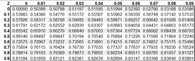
Here, you can see the z-scores at different alphas. Here, if we test at alpha = 0.05, the test statistics rejects the null hypothesis if the z-score is greater than 1.645 or less than -1.645. Another way we can test our hypothesis is by looking at the p-value of the z-score on a z-table. If it is less than 0.05, we reject the null hypothesis. A z-table generally looks like the image below.
One Tailed Hypothesis Test Example
To test our null hypothesis in the example with wait times, we have to find the z-score in the left tail z-table below.
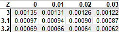
With a p-value of 0.00135, which is less than 0.05, we reject the null hypothesis of a wait time of 5 minutes.
Did you like this article? Rate it!


