Chapters
In previous sections, you learned about the fundamentals of descriptive statistics. Specifically, you learned about the properties of measures of central tendency and variability and how they describe the characteristics of distributions. Here, we’ll review the various distributions you will encounter in the probability theory as well as their properties.
Random variables in statistics are variables that can take on any value based on a probability distribution. As you learned in previous sections of this guide, probability distributions, like the normal distribution, tell you how typical a value is given measures like the mean and standard deviation.
Typical values are another way of saying values that are probable and improbable. The classic illustration of a random variable is the flip of a coin. Let's call the flip of a coin X, where the result, which can be either heads or tails, is what makes our random variable random. Here, the probability that it will be heads is 0.5, or 50%.
There are two types of numbers, as we discussed before: discrete and continuous variables. The differences between the two can be summarized in the table below.
| Discrete | Continuous | |
| Definition | Can take on a finite amount of possibilities | Can take on an infinite amount of possibilities |
| Example | Colour: Blue, Red, Yellow | Height: 1.69 cm, 1.692 cm, 1.693…..9cm |
| Characteristics |
|
|
If a random variable is a discrete variable, it takes on a discrete distribution and, likewise, if a random variable is continuous, it takes on a continuous distribution.

Discrete Distributions
As we mentioned, random variables which are discrete take on discrete distributions. Distributions are nothing more than the probability of a random variable’s outcome. Therefore, a discrete distribution is nothing more than a discrete probability distribution. In other words, a discrete probability distribution displays each outcome of a random variable and its probability of occurring.
There are three fundamental discrete distributions: binomial, geometric and Poisson distributions.
Binomial
Binomial distributions deal with binomial variables, which are variables that can take on only two values. Think of our example before, with our random variable X of flipping a coin. This X could take on only two values: heads and tails.
We can generalize any random variables with two outcomes as being either 0 or 1, where we assign each outcome either a 0 or a 1. The table below is a list of the most common binomial variables, also called Boolean variables.
| Outcome 1 | Outcome 2 |
| Heads | Tails |
| Yes | No |
| True | False |
| Success | Failure |
| 1 | 0 |
The binomial distribution can be written in the following format,
[
X backsim B(n,p)
]
This format is how all distributions are written, were a random variable is said to follow a distribution, signalled here by a “B,” and where  and
and  are the parameters. The parameter is the number of observations, or sample size, and p is the probability of either outcome 1 or outcome 2 occurring.
Naturally, if was equal to the probability of outcome 1, then the probability for outcome 2 would be,
[
q = 1 - p
]
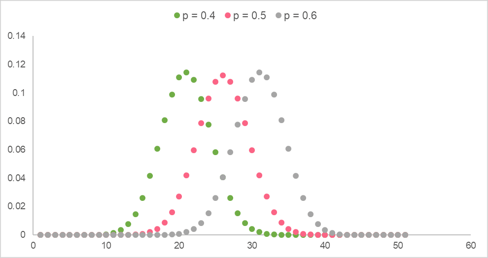
The image below shows binomial distributions for several and .
Geometric
Geometric distributions deal with geometric sequences, which is where each number in the sequence can be found by multiplying the previous number by some fixed constant. This is because the geometric distribution is a probability distribution that indicates the probability of a certain amount of failures before the first success.
The table below illustrates the assumptions that need to be met about a variable in order to use a geometric distribution.
| Assumption | Example |
| The outcome of the random variable being studied is found after a series of independent trials | The random variable being studied is people’s favourite ice cream flavour at a local ice cream shop |
| There are only two outcomes for the random variable, either a failure or a success | There are only two flavours, vanilla and chocolate, where we deem vanilla a “failure” and chocolate a “success” |
| The probability for a success is the same in every independent trial | The probability of someone liking vanilla is the same for every independent trial because one person preferring vanilla has no effect on whether the next person you ask likes vanilla |
The geometric distribution is written as,
[
X backsim geom(p)
]
Below, you’ll find several geometric distributions with different .

Poisson
Poisson distributions deal with the outcome of a random variable within a specific time frame, where it depicts the probability for each number of times an outcome can occur within that time interval. Below, you can find the assumptions for a Poisson distribution.
| Assumption | Example |
| The number of times an event occurs can take on only integer values |  , the number of times an outcome occurs, can only = 0, 1, 5, 100, etc. , the number of times an outcome occurs, can only = 0, 1, 5, 100, etc. For example, the number of times someone calls customer service |
| The outcomes are independent | One person choosing to call customer service does not affect another person choosing to call customer service |
| Outcomes cannot happen at the exact same time | Think about it - even if you place a call at the same time as another customer, there will be milliseconds of difference between the time they connect to customer service |
Poisson distributions are written as,
[
X backsim Pois(mu)
]
Where the mean,  , is the average number of events occurring in the interval given by,
[
mu = lambda t
]
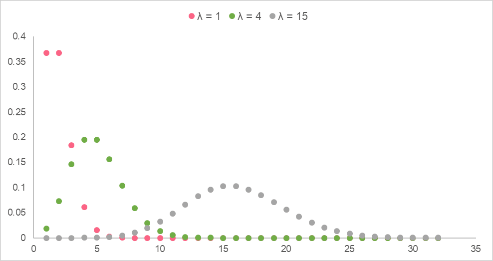
Below are Poisson distributions with different 
| Discrete Distributions | ||
| Binomial | Geometric | Poisson |
| Deals with Boolean variables: ones that only take on two values | Variables in a geometric sequence, where the probability is of the first “success” | Indicates the probability of an event occurring a certain amount of times in a given time frame. |
Example:
| Example:
| Example:
|
| [ X backsim B(n,p) ] | [ X backsim geom(p) ] | [ X backsim Pois(mu) ] |
Continuous Distributions
As the name suggests, continuous distributions display the probability of continuous random variables. These can be variables like heights, test scores, speed, etc. While there are a couple of basic distributions, the most important one to know is the normal or standard normal distribution.
Normal
As we’ve showed you before, the normal distribution models normal variables, which follow the 68-95-99.7 rule. The properties for a normal distribution are listed in the table below.
| Property | Explanation |
| Shape | A normal probability distribution is shaped like a bell curve, which is why it’s often called a “bell curve” |
| Distribution | Its distribution is symmetric around the mean, which means the two sides before and after the mean mirror each other |
| Rule | 68% of the data falls within 1  of the mean of the mean 95% of the data falls within 2 99.7% fall within 3 |
It is written as,
[
X backsim N(mu, sigma)
]
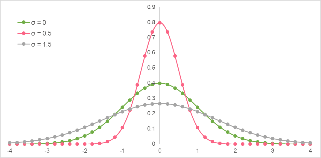
Below are normal distributions with different  .
.

Standard Normal
A standard normal distribution is the same as a normal distribution. The only difference is that the data points are standardized using the standardization, or z-score, formula.
[
A = frac{X-mu}{sigma}
]
It is written as,
[
X backsim N(0, 1)
]
Below is a standard normal distribution. Notice that the mean is always at 0.
| Continuous Distributions | |
| Normal | Standard Normal |
| Models continuous variables with a normal distribution | Models continuous variables that have been standardized |
| [ X backsim N(mu, sigma) ] | [ X backsim N(0, 1) ] |
Did you like this article? Rate it!


Can you help me answer my activities