Chapters


Measures of Central Tendency
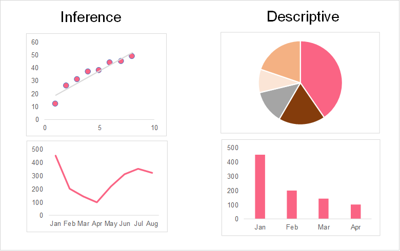
While statistics can often be thought of as one general clump of metrics and data, there are actually two major branches within the field. These two distinct branches are: inferential and descriptive statistics. Inferential statistics involve the tools and methods used to predict the future using the data that you have. Descriptive statistics, on the other hand, involve using methods and crafting visualizations that describe the data set.
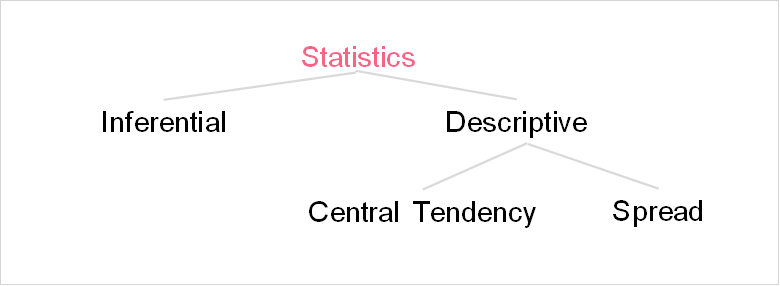
Within descriptive statistics, there are two types of measures that you can calculate: measures of central tendency and spread. Confusing right? The image below maps out the subjects we’ve discussed so far.
Measures of central tendency are descriptive statistics that tell us about the location of the centre of the data set. These generally involve the mean, median and mode. The table below gives their definitions and formulas
| Measure | Definition | Example | Formula |
| Mean | The average of a variable | The average amount of rain in a year |  |
| Median | The middle point of a variable | The median salary is 13,000 pounds | Order data from least to greatest, pick the middle |
| Mode | The most frequently occurring value of a variable | The mode dessert of a restaurant is cake | Calculate the frequency and pick the one with the highest frequency |
Measures of Spread
In contrast to measures of central tendency, measures of spread are descriptive statistics that can help us understand how far spread the data is around the centre point. As you can see, measures of spread work hand in hand with measures of central tendency. You cannot talk about measures of spread without the mean, median or mode.
The three major types of spread measures are the standard deviation, variance and range. A definition, formula and example for each can be found in the table below.
| Measure | Definition | Example | Formula |
| Standard deviation | How far spread apart the data is from the mean | The standard deviation of running times is 3.4 seconds |  |
| Variance | The variance is the average amount between all observations and the mean | The variance of running times is 11.56 seconds squared |  |
| Range | The difference between the highest and lowest values in a variable | The range in running times is 60 seconds | 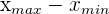 |
Median Definition
Recall that the median is actually one of the measures of central tendency. The median is defined as the middle point of a variable. Because the median is considered to be the midpoint of a variable, it is the exact point that represents a separation between the upper half and lower half of the values within a variable.
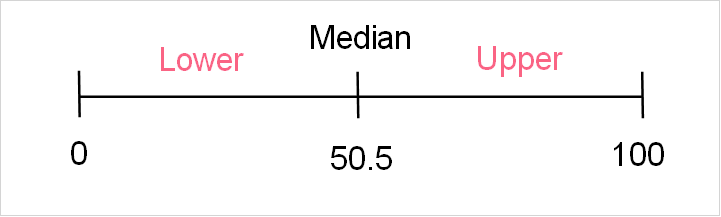
Take, for example, a variable that goes from 0 to 100. The middle point of this variable would be 50.5, where everything above 50.5 would represent the upper half of the data and everything below it would represent the lower half.
How to Find the Median
Finding the median is quite simple. While there are several formulas you will find for the median, the easiest way to calculate it is to do it by hand. The following table goes through each step in finding the median.
| Step | Description | Example |
| 1 | Start with one variable with numerical values | 1,4,6,9,2,6,8 |
| 2 | Order the values from least to greatest | 1,2,4,6,6,8,9 |
| 3 | Extract the middle value if there are an odd number of observations for the variable | 6 |
In the example above, there are 7 observations for the variable. In order to extract the middle number, you simply eliminate each number from each end until you reach the middle. The image below demonstrates how this is done.

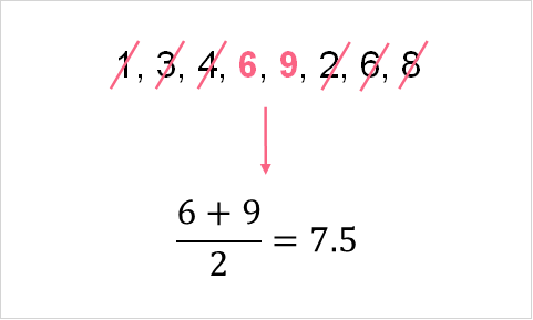
However, when you have a variable with an even number of observations the calculation is a bit different. Instead of only one value in the middle, there are two. So, instead of taking just the middle value, you take the average of the two numbers in the middle. Let’s add a 3 to the data set above and see how that changes the calculation.
Median Example
This section will give a step by step example of finding the median. Let’s start with a practice data set. The following table has the amount of time it takes to go from 0 to 60 miles per hour, a common benchmark for automobile performance.
| No. | Car | 0-60mph |
| 1 | Porsche 918 Spyder | 2.1 |
| 2 | Lamborghini Diablo SE | 4.0 |
| 3 | Bugatti Veyron | 2.5 |
| 4 | BMW 6 Series 4.4 V8 | 3.8 |
| 5 | Ferrari 488 Pista | 2.7 |
| 6 | Honda NSX | 3.0 |
| 7 | McLaren 720S | 2.5 |
| 8 | Jaguar F Type R | 3.9 |
| 9 | Tesla Model S P 100D | 2.28 |
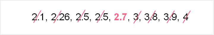
Following the steps from the previous table, the first step in finding the median is to order the values from least to greatest. After sorting the list, you then find the median by eliminating a number from each side until reaching the middle. Because this variable has an odd number of observations, we expect there to be only one number in the middle.
When to Use the Median
The median should be used instead of the mean whenever your data set is highly skewed. Take the previous data set as an example, adding a few more cars to the list.
| No. | Car | 0-60mph |
| 1 | Porsche 918 Spyder | 2.1 |
| 2 | Lamborghini Diablo SE | 4.0 |
| 3 | Bugatti Veyron | 2.5 |
| 4 | BMW 6 Series 4.4 V8 | 3.8 |
| 5 | Ferrari 488 Pista | 2.7 |
| 6 | Honda NSX | 3.0 |
| 7 | McLaren 720S | 2.5 |
| 8 | Jaguar F Type R | 3.9 |
| 9 | Tesla Model S P 100D | 2.28 |
| 10 | Renault 25 2.5 V6 | 7.9 |
| 11 | Subaru BRZ 2L | 7.9 |
The mean time is about 3.87 seconds, while the mean without the last two observations is 2.98. This is almost a full second more, which doesn’t give us that accurate of a picture, as most of the data is below 3.87. Instead, we could use the median, which is 3, to represent the centre of the data.

Did you like this article? Rate it!


Using facebook account,conduct a survey on the number of sport related activities your friends are involvedin.construct a probability distribution andbcompute the mean variance and standard deviation.indicate the number of your friends you surveyed
this page has a lot of advantage, those student who are going to be statitian
I’m a junior high school,500 students were randomly selected.240 liked ice cream,200 liked milk tea and 180 liked both ice cream and milktea
A box of Ping pong balls has many different colors in it. There is a 22% chance of getting a blue colored ball. What is the probability that exactly 6 balls are blue out of 15?
Where is the answer??
A box of Ping pong balls has many different colors in it. There is a 22% chance of getting a blue colored ball. What is the probability that exactly 6 balls are blue out of 15?
ere is a 60% chance that a final years student would throw a party before leaving school ,taken over 50 student from a total of 150 .calculate for the mean and the variance
There are 4 white balls and 30 blue balls in the basket. If you draw 7 balls from the basket without replacement, what is the probability that exactly 4 of the balls are white?