Chapters


Three Basic Types of Means
Types of Means
When people think of data sets, they tend to think of orderly data that follows common patterns such as a normal distribution. The reality, fortunately for us statisticians, is much more complex than that. As you learn about relationships between numbers in some higher-level maths courses, you start to learn that not every relationship is a linear relationship.
A linear relationship is one that follows an additive pattern between numbers. Additive simply means that you simply need to add or subtract a certain function from one number to arrive to the next one. This can be exemplified by a linear function such as,
\[
2x +3
\]
Let’s say we have this relationship for the following numbers:
| Value | Linear Relationship |
| 5 | (2*1)+3 |
| 7 | (2*2)+3 |
| 9 | (2*3)+3 |
| 11 | (2*4)+3 |
| 13 | (2*5)+3 |
While the most common way to graph this function would be on an axis, like below
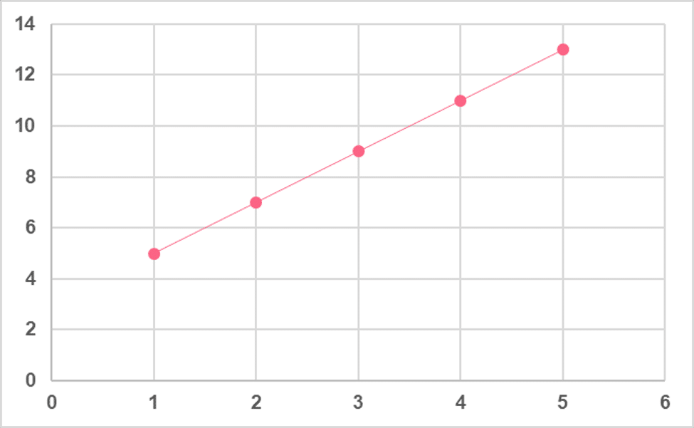
Arithmetic Mean
The arithmetic mean, also known as AM, is the mean you’ve learned in previous sections of this guide. It is a simple average found by summing all observations and dividing by the number of observations, taking the form of the following formula
\[
\frac{\Sigma x_{i}}{n}
\]
Taking from our previous example, we would use the arithmetic mean to calculate the mean, which would lead us to the following result.
\[
\dfrac{5+7+9+11+13}{5}
\]
\[
\dfrac{45}{5}
\]
\[
9
\]
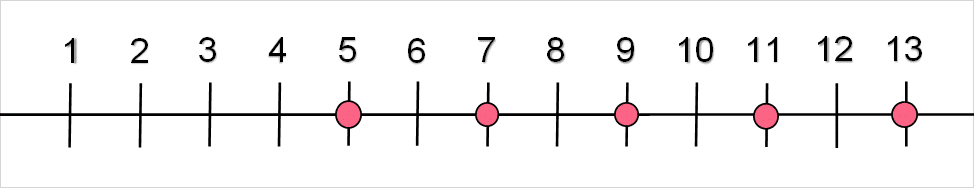
Taking a look back at our line plot, we can see that the mean corresponds to the exact midpoint of our data. This signals to us that using the AM here is appropriate because it is a good representation of the centre of our data.
Geometric Mean
In the previous example, we found the mean for a relatively simple relationship. Many of your data sets will have variables that are linear, or additive. However, there are many instances where you will either receive variables or transform your variables into ones that have a multiplicative or exponential relationship.
For example, many people have to transform the variables in their data set in order to better interpret their data or to simply lend them a more normal distribution. In this case, it wouldn’t make sense to use the AM because it wouldn’t truly reflect the centre of the data. To illustrate this point, let’s take the previous example and multiply each number by 2 consecutively.
| Value | Multiplicative Relationship |
| 5 | 5*2 |
| 10 | 10*2 |
| 20 | 20*2 |
| 40 | 40*2 |
| 80 |
Here, taking the AM would result in the following,
\[
\dfrac{5+10+20+40+80}{5}
\]
\[
\dfrac{155}{5}
\]
\[
31
\]
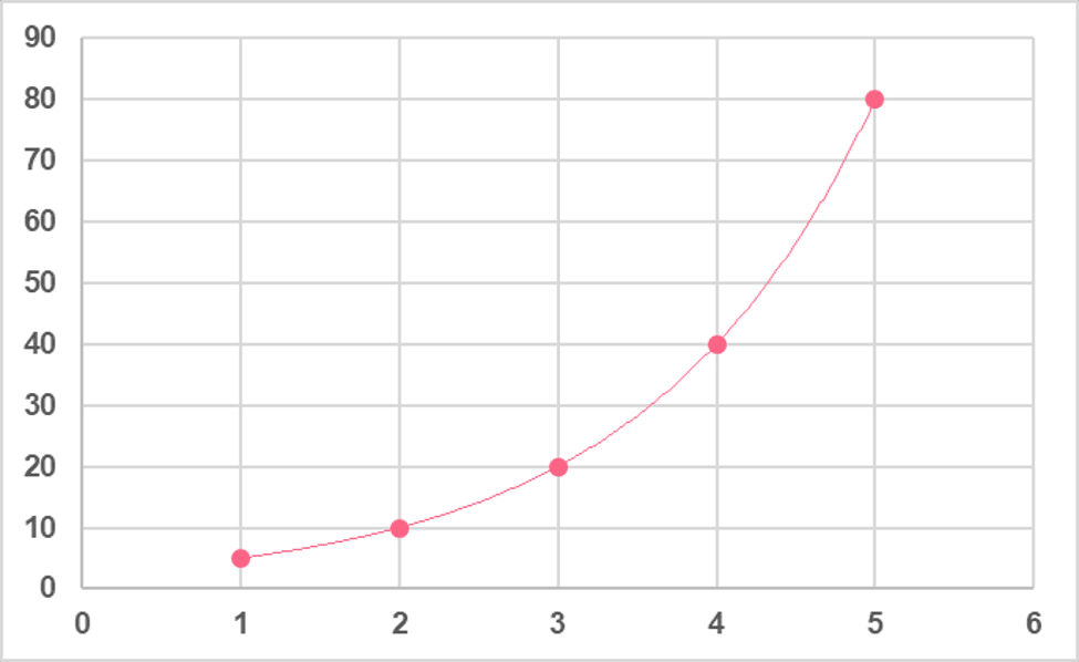
Plotting this on an axis, shown in the image below, we see that now we approach a graph with a curved line, also known as a geometric series.

\sqrt[n]{a_{1}*a_{2}*\dotsm*a_{n}}
\]
Where we take each number in our data set and multiply them, then take the nth root of this multiplied value. The nth root indicates the sample size, or  , of our data set.
This means that our result would be ,
\[
\sqrt[5]{5*10*20*40*80}
\]
\[
\sqrt[5]{3 \thickspace 200 \thickspace000}
\]
\[
20
\]
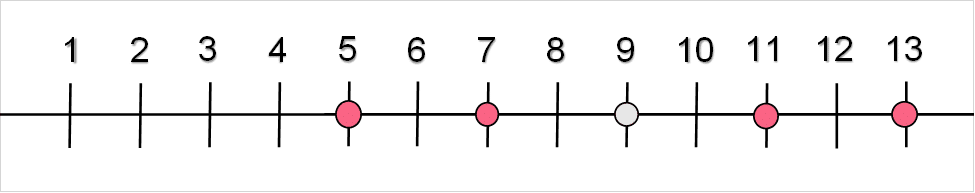
Here, we can see that the geometric mean is actually equal to the median, which is the middle point of our data. Looking at the line plot below, we can see this is much closer to the centre point of our data set than the AM.

Harmonic Mean
The harmonic mean is the third type of mean and probably the one you will either use the least or not at all. Also known as the HM, this mean uses reciprocals to calculate the relationship between fractions.
As a reminder, a reciprocal is basically 1 divided by a number, or  , which basically equates to the numerator and denominator trading places. For example,
\[
\dfrac{4}{1} = \dfrac{1}{4}
\]
Or,
\[
\dfrac{2}{3} = \dfrac{3}{2}
\]
The formula for the HM is a bit complicated, as you can see below.
\[
H = \frac{n}{\dfrac{1}{x_{1}} + \dfrac{1}{x_{2}} + \dotsm + \dfrac{a}{x_{n}}}
\]
\[
= \frac{n}{\Sigma_{i=1}^{n}{\dfrac{1}{x_{i}}}}
\]
Don’t worry about not understanding the intricacies of this formula, chances are you’ll probably never need it. It’s helpful to see, however, and to know that there are three Pythagorean Means.
Problem 1: Choosing Which Mean to Use
As we’ve learned, when calculating the mean, there are generally three basic types of means from which to choose from. While we’ve guided you through scenarios that involve both the arithmetic and geometric mean, in real life you’ll rarely have someone telling you which one is the correct one to use.
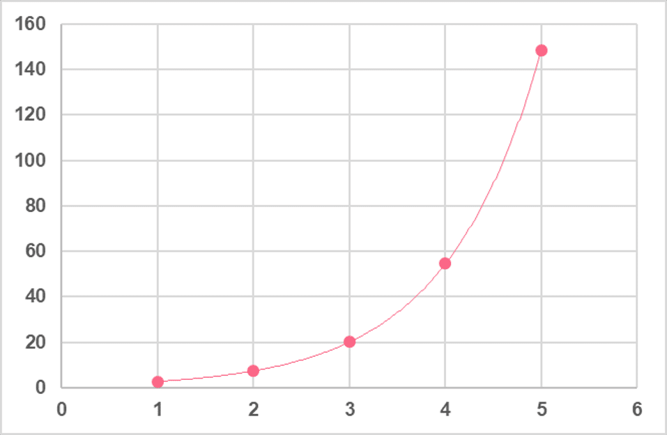
Given the following data table, decide which mean would be more appropriate to use by describing the type of relationship there exists between the data points. Then, calculate it.
| Observation | Value |
| 1 | 3 |
| 2 | 7 |
| 3 | 20 |
| 4 | 55 |
| 5 | 148 |
Solution to Problem 1
In this problem, we were tasked with:
- Describing the relationship between the data points
- Choosing which mean formula to use
- Calculate the mean
As we can see from the values, there is no clear linear relationship between them, which suggests a multiplicative relationship. This becomes even more apparent when we graph the numbers.
| Step | Calculation |
| 1. Multiply all the values in the data set | \[ 3*7*20*55*148 = 3 \thickspace 269 \thickspace 017 \] |
| 2. Take the nth root of this multiplied number | \[ \sqrt[5]{3 \thickspace 269 \thickspace 017} = 20 \] |
Did you like this article? Rate it!


Can you help me answer my activities