Chapters


First Derivative
In calculus, the most common operation you will perform is taking the derivative of a number. Take the following equation as an example.

Let’s plug in some numbers into this function and then plot it to get some more information about its shape.
| x |  |  |  | d + e - f + 10 |
| 1 | 4 | 5 | 6 | 13 |
| 2 | 16 | 20 | 24 | 22 |
| 3 | 36 | 45 | 54 | 37 |
| 4 | 64 | 80 | 96 | 58 |
| 5 | 100 | 125 | 150 | 85 |
| 6 | 144 | 180 | 216 | 118 |
Plotting this onto a graph, we get:

When we plot the graph, we get important information such as:
- Where the function increases and decreases
- How fast it is increasing and decreasing at certain points
For example, at x equal to 5, we can see the function is increasing rapidly given the slope is quite steep at that point. While graphing gives us useful information, it is not practical to graph every equation in order to extract information from it.
Taking the derivative of a function solves this problem. The derivative of a function is a measure of how fast or slow the function is increasing or decreasing at any given point in the function. This is also known as the rate of change.
First Derivative Properties
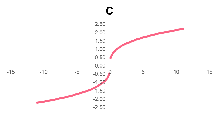
The most important property of taking the derivative of a function is something known as continuity. Take a look at the examples below to get an idea of what being continuous means.
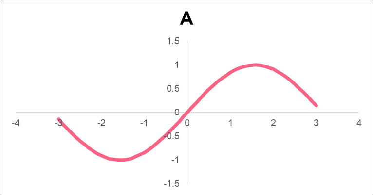

| A | Continuous | No breaks in the line |
| B | Not Continuous | A break |
| C | Not Continuous | A hole |
Critical Point
Take any random point on the graph of a continuous function as an example. If the first derivative at that point is zero, that point is a critical point of the function. In formal terms:

Let’s see what this translates into. We know that the first derivative is the rate of change of a function. If the first derivative is equal to zero, this is like saying there is no change at that point.

As you can see, there are two points on the graph where the rate of change appears to be zero. We can see this by drawing the slopes at each point. At points A and C, the slope looks flat. Compare this to point B, where the slope is diagonal.
Rolle’s Theorem
Rolle’s theorem is an important theorem because it helps you understand the mean value theorem. Rolle’s theorem states the following:
| Assumption 1 | If you have a function that: | |
| Sub-condition | Is continuous on an interval [x,y] | |
| Sub-condition | Can be differentiated on the interval (x,y) | |
| Sub-condition | The function at x - f(x) - is equal to the function at y - f(y) | |
| Assumption 2 | There is a point z where f’(z) = 0 | |
| Result | Then the function has a critical point in the interval (x,y) |
Which is basically saying that between these two points there is a critical point if these conditions are satisfied.
Mean Value Theorem
The mean value theorem is similar to Rolle’s theorem, except that it actually needs Rolle’s theorem in order to prove that it exists. The MVT says the following.
| Assumption 1 | If you have a function that: | |
| Sub-condition | Is continuous on an interval [x,y] | |
| Sub-condition | Can be differentiated on the interval (x,y) | |
| Result | There is a point z where f’(z) is  |
Problem 1
The owner of a shop wants to know more about the influence of the changes in the average price of the goods in their store on the demand. You have the following function:

This function details the price and demand of the store. In order to give the owner more information, you decide to tell them at which price the demand stops increasing or decreasing. In other words, you want to find the relative extrema at this point, if there are any. Solve this problem.
Problem 2
You are interested in the following function.

Conduct a first derivative test for local extrema. Then, plot the function onto a graph, marking the extrema.
Problem 3
You are given the following information.
| Function | f(x) |
| Point 1 | Continuous on [4,10] |
| Point 2 | Differentiated on [4,10] |
| Point 3 | f(4) = -1 |
| Point 4 | f’(x)  8 8 |
Using the mean value theorem, what is the biggest value f(10) can take on?
Solution Problem 1
In order to find the point at which the price stops increasing or decreasing, we need to differentiate the equation and solve for where y will be equal to zero.
First, we need to apply the rule that deals with adding or subtracting two functions.

This tells us that the first derivative of two functions added or subtracted from each other is the same as the sum or difference of the first derivative of each separate function.

The first derivative of a constant is 0, so we are left with :

Which means that the demand doesn’t change when the price is zero.
Solution Problem 2
For this equation, we were asked to conduct a first derivative test to find local extrema. First, we need to take the first derivative of the equation.


Now, we simply see which value of y where x is equal to zero.
\[
y = 2x^{3} + 4
\]
\[
y = 2(0^{3}) + 4
\]
\[
y = 0 + 4 = 4
\]
The point (0,4) is a candidate for local extrema.
Solution Problem 3
For this problem, we simply conduct the MVT backwards.
\[
f(10) - f(4) = f’(z)(10 - 4)
\]
\[
f(10) = f’(z)(10 - 4) + f(4)
\]
\[
f(10) = 6(f’(z)) -1
\]
Since f’(z) 8, we know that the highest number that z can be is 8.
\[
f(10) = 6(8) -1 = 47
\]
Did you like this article? Rate it!


