Chapters


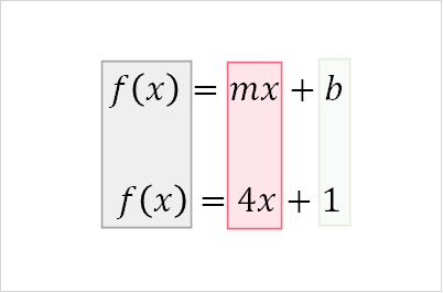
Linear Function
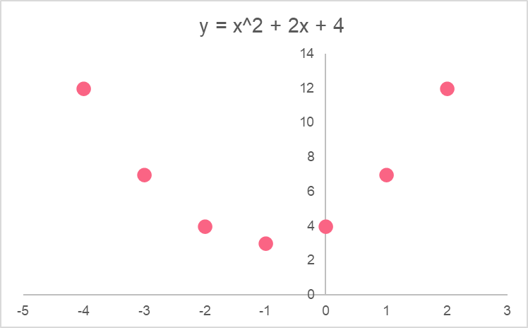
In order to graph a linear function, it’s enough to simply plug in values for x to get a resulting y value. Taking the example from the image above, let’s take these values of x as an example:
| x | y |
| 1 | 5 |
| 2 | 9 |
| 3 | 13 |
| 4 | 17 |
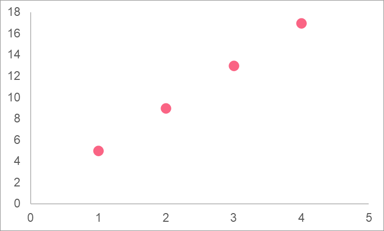
A linear function represents a straight line relationship. As you can see in the graph, this means that the variables x and y have a linear relationship with each other.
Polynomial Function
Polynomial functions are the most common functions you’ll encounter in calculus. In order to understand what a polynomial is, let’s take a look at a monomial.
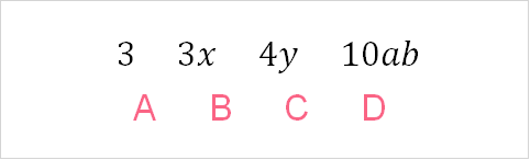
| A | B | C | D |
| Constant | Constant and x variable | Constant and y variable | Constant and b and a variables |
The monomial is the basic building block of the polynomial. It can be either a constant or a constant with any variables. What happens when there is more than one monomial, like we have in the linear equation?

Let’s break down different types of polynomials to find out.
| Definition | Explanation | |
| Monomial | Made up of one monomial | Mono = one |
| Binomial | Made up of two monomials | Bi = two |
| Trinomial | Made up of three monomials | Tri = three |
| Polynomial | Made up of monomials | Poly = many |
Here is an example of each type of polynomial:
| Monomial |  |
| Binomial |  |
| Trinomial | 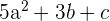 |
| Polynomial |  |
You can call any combination of monomials polynomials.
Absolute Extrema
Now that we’ve covered the basics of polynomials, we can take a look at the most important concept in optimization: extrema. In order to understand absolute extrema, let’s take a parabola as an example:

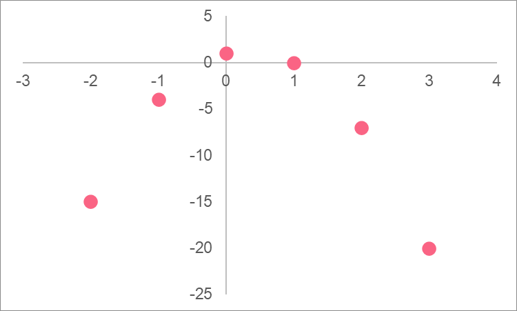
Based on the graph, it is easy to pinpoint where the maximum, or vertex, of the parabola is. However, what if we have more than one point that can be the maximum or minimum?
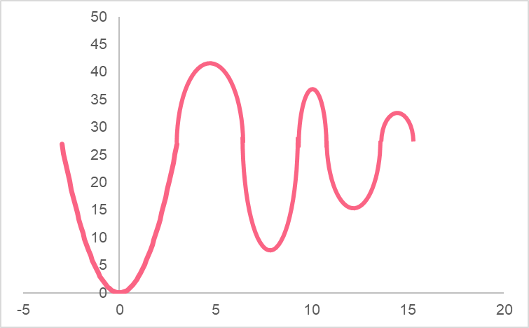
In this case, what would be the maximum? In many situations, functions have multiple points that can be considered maxima or minima. These points are known as extrema:
| Extrema | Minima or maxima | Any low or high point on the graph |
| Absolute Extrema | Minima or maxima | The highest or lowest point on the graph |
The absolute extrema are defined as the extrema that, within the domain specified, are the highest or lowest. In other words, when we look at a specific range of values for a function, the absolute extrema are the highest or lowest points in that range.
| A | Absolute maximum | The highest point in a range |
| B | Absolute minimum | The lowest point in a range |
Relative Extrema
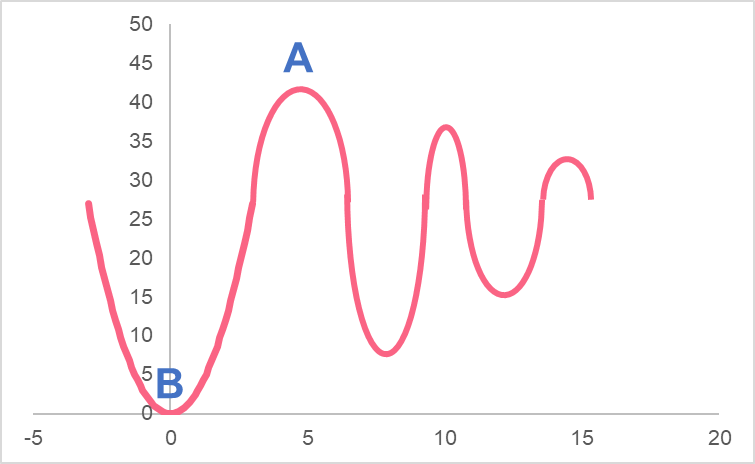
Relative extrema are different from absolute extrema because they are not the highest or lowest point in the range, but rather every minimum and maximum between those points.
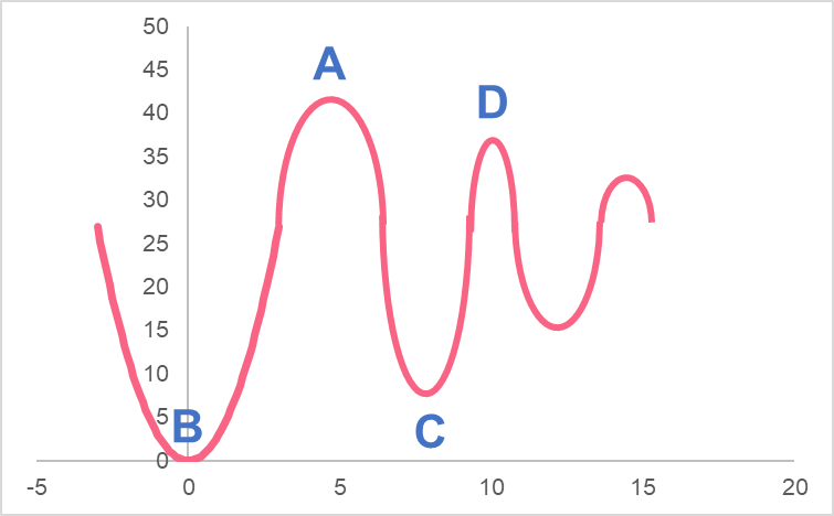
| A | Absolute maximum | The highest point in a range |
| C | Relative minimum | A minimum between the absolute extrema |
| D | Relative maximum | A maximum between the absolute extrema |
| B | Absolute minimum | The lowest point in a range |
Here, we can see that while the two ending points are absolute extrema, the two points in the middle are relative extrema.
Optimization
Optimization in calculus involves finding the absolute extrema within a range. What this means is that we want to perform a first derivative test to find the absolute minimum or maximum. We do this for two reasons.
| Minimize dimension | Absolute minimum |
| Maximize dimension | Absolute maximum |
| Maximize profit | Absolute maximum |
| Minimize cost | Absolute minimum |
First Derivative Test
In order to find the absolute extrema, we first take the first derivative of a function and then solve for x. Take the following as an example.
| First derivative | 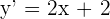 |
| Rearrange for x |  |
| Solve for x |  = -1 = -1 |
Calculus Fence Problem
A common optimization problem is the following. A homeowner wants to build a fence with 100 meters of fencing for their backyard. What is the largest area of a rectangular field?

The area and perimeter of a rectangle is as follows:
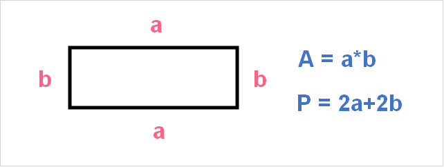
Because we have the total, in other words maximum, length of the fence, we can replace this into the formula.
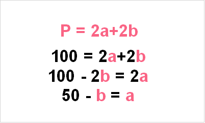
Now that we have the value for a, we can replace this into our formula for area.

Now that we have the formula for the area of our fence, we can use the first derivative test to find the maximum.

Now that we have the maximum width of the fence, we can get the length and the maximum area.

Calculus Volume Problem
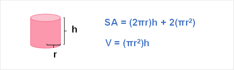
Another common problem in optimization deals with cylinders. For example, you have 300 millilitres of juice. You need to find the dimensions of a cylindrical can that would minimize the cost of producing that can.
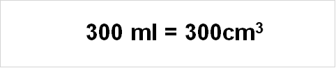
300 ml are equal to 300 cubic centimetres. Let’s take a look at the surface area and volume equations for a cylinder.
We want to minimize the surface area. Since we know the final volume that has to fit into the cylinder, we can replace this in the formula. Then, we re-arrange the formula so that only one variable is on each side.

Now that we have the height, we can plug this into the surface area equation.

Then, we perform a first derivative test.
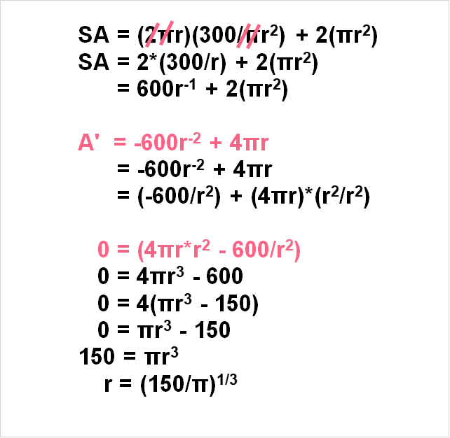
Now that we have r, we can find h by plugging it back into the equation.

Now we have the dimensions for the can that would minimize the cost.
Did you like this article? Rate it!


